Introduction In Lecture 2 we established the following fundamentals - PDF document
Massachusetts Institute of Technology Department of Electrical Engineering and Computer Science 6.453 Quantum Optical Communication Lecture Number 3 Fall 2016 Jeffrey H. Shapiro c 2006, 2008, 2012, 2015 Date: Thursday, September 15, 2016
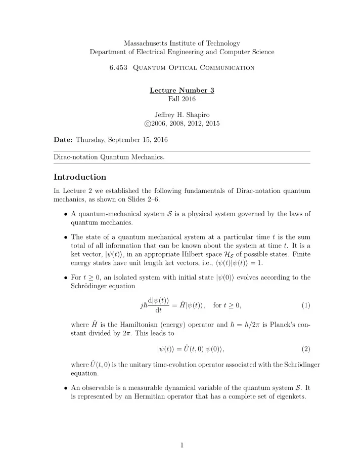
Massachusetts Institute of Technology Department of Electrical Engineering and Computer Science 6.453 Quantum Optical Communication Lecture Number 3 Fall 2016 Jeffrey H. Shapiro � c 2006, 2008, 2012, 2015 Date: Thursday, September 15, 2016 Dirac-notation Quantum Mechanics. Introduction In Lecture 2 we established the following fundamentals of Dirac-notation quantum mechanics, as shown on Slides 2–6. • A quantum-mechanical system S is a physical system governed by the laws of quantum mechanics. • The state of a quantum mechanical system at a particular time t is the sum total of all information that can be known about the system at time t . It is a ket vector, | ψ ( t ) � , in an appropriate Hilbert space H of possible states. Finite S energy states have unit length ket vectors, i.e., � ψ ( t ) | ψ ( t ) � = 1. • For t ≥ 0, an isolated system with initial state | ψ (0) � evolves according to the Schr¨ odinger equation j � | ψ ( t ) � d ˆ = H | ψ ( ) � , t for t ≥ 0, (1) d t ˆ where H is the Hamiltonian (energy) operator and � = h/ 2 π is Planck’s con- stant divided by 2 π. This leads to ˆ | ψ ( t ) � = U ( t, 0) | ψ (0) � , (2) ˆ where U ( t, 0) is the unitary time-evolution operator associated with the Schr¨ odinger equation. • An observable is a measurable dynamical variable of the quantum system S . It is represented by an Hermitian operator that has a complete set of eigenkets. 1
• For a quantum system S that is in state | ψ ( t ) � at time t , measurement of the observable ˆ � O = o n | o n �� o n | , (3) n where {| o n �} are the observable’s orthonormal eigenkets and { o n } are its asso- ciated eigenvalues (assumed to be distinct), yields an outcome that is one of these eigenvalues according to the probability distribution Pr( o n ) = |� o n | ψ ( t ) �| 2 . (4) If the observable that is measured has a continuum of non-degenerate eigenval- ues, so that � ∞ ˆ O = d o o | o �� o | , (5) −∞ where the associated (infinite-length) orthonormal eigenkets are {| o �} , then the probability density for obtaining the outcome o is p ( o ) = |� o | ψ ( t ) �| 2 . (6) Today we will complete our foundational work on Dirac-notation quantum mechanics. We begin by continuing our treatment of quantum measurement statistics. Moment Equations for Quantum Measurements Probability mass functions and probability density functions provide complete sta- tistical characterizations of discrete and continuous classical random variables, re- spectively. However, for many applications more limited—and hence incomplete— statistics will suffice. In particular, if x is a real-valued classical random variable, then its mean value � � n X n Pr( X n ) , for x discrete valued � x � = (7) � d X Xp ( X ) , for x continuous valued , gives us useful information about the deterministic part of x , i.e., its signal compo- nent. The deviation of x from its mean, ∆ x ≡ x − � x � , (8) is then the random (noise) component of x . It is a zero-mean random variable whose mean-squared strength is the variance of x , n ( X n − � x � ) 2 Pr( X n ) , � � for x discrete valued var( x ) = � ∆ x 2 � = (9) � d X ( X − � x � ) 2 p ( X ) , for x continuous valued . 2
� By the linearity of expectation—which you are familiar with from your probability prerequisite—we have that var( x ) = � x 2 � − � x � 2 , (10) a relation that we will use from time to time in performing variance calculations. Although knowledge of the mean and variance of x is far less information about its statistics than knowing its full characterization, it is nonetheless sufficient to evaluate the signal-to-noise ratio, � x � 2 SNR ≡ , (11) var( x ) which gives us a quantitative measure of how noisy this random variable is. In particular, the Chebyschev inequality from probability theory can be cast in the following form: �� � � � x − � x � � ≥ δ � � ≤ 1 /δ 2 SNR , Pr for � x � = 0 and any δ > 0 . (12) � x � � � Thus, for example, a random variable with a 60 dB SNR (SNR = 10 6 ) has at most a 1% probability of being more than 1% away from its mean value. 1 In light of the preceding remarks, you should not be surprised that much of our study of quantum measurement statistics will be limited to mean values and variances. To see how to simplify the calculations of these moments for observable measurements ˆ we turn to Slide 7. Suppose O has a discrete eigenvalue spectrum, with distinct ˆ eigenvalues. The mean value of the O measurement at time t is then o n |� o n | ψ ( t ) �| 2 = � ˆ � � � O � ≡ o n Pr( o n ) = o n � ψ ( t ) | o n �� o | ψ ( t ) � (13) n n n n �� � ˆ = � ψ ( t ) | o n | o n �� o n | | ψ ( t ) � = � ψ ( t ) | O | ψ ( t ) � , (14) n so that it can be calculated without explicitly evaluating Pr( o n ). You should verify that higher-order moments for this observable can be found via, 2 � ˆ � n Pr( o n ) = � ψ ( t ) | ˆ O k � ≡ o k O k | ψ ( t ) � , for k = 2 , 3 , . . . , (15) n and thus = ∆ O 2 � = � O 2 � − � O � 2 = � ψ ( t ) | O 2 | ψ ( t ) � − � ψ ( t ) | O | ψ ( t ) � 2 . ˆ ˆ ˆ ˆ ˆ ˆ var( O ) � (16) 1 The Chebyschev inequality is very general, and so it is very weak. If x is a Gaussian random 2 variable, then we have that the probability in (12) is no more than e − δ SNR / 2 , which is far smaller than 1 /δ 2 SNR when δ 2 SNR ≫ 1. To do so you will want to show that O k = ˆ 2 n o k � n | o n �� o n | , which follows from the eigenket- ˆ eigenvalue relation for O . 3
The corresponding results for an observable whose eigenvalue spectrum is the contin- uum −∞ < o < ∞ and non-degenerate are found in a similar manner, 3 � ∞ ∞ � � ˆ O k � d o o k p ( o ) = d o o k |� o | ψ ( t ) �| 2 = (17) −∞ −∞ � ∞ ∞ �� � d o o k � ψ ( t ) | o �� o | ψ ( t ) � = � ψ ( t ) | d o o k | o �� o | = | ψ ( t ) � (18) −∞ −∞ � ψ ( t ) | ˆ O k | ψ ( t ) � , = for k = 1 , 2 , 3 , . . . (19) From this result it follows that Eq. (16) can also be used for observables whose eigenvalue spectra are continuous. Schr¨ odinger versus Heisenberg Pictures First treatments of quantum mechanics—including what we have done so far—almost invariably take the Schr¨ odinger equation route to characterizing the time evolution of a quantum system. Here, for an isolated system, the state vector evolves in time but the observables are time-independent operators. Ultimately, we’d like to have ap- propriate quantum versions for Maxwell’s equations. Here, the electric and magnetic fields should be (3-D vector) observables that evolve in space and time. Then, for a quantized electromagnetic wave propagating in a source-free region of empty space, we would expect that the state vector should be constant if no measurements are made. We can convert our Dirac-notation quantum mechanics to an approach that has observables evolving in time and state vectors that are constants by going to the Heisenberg picture. We’ll make that change today, after which we will stick with the Heisenberg picture for the rest of the semester. Consider the descriptions given on Slide 8 for the Schr¨ odinger and Heisenberg pictures of an isolated quantum system S for t ≥ 0. The Schr¨ odinger picture has ˆ ˆ time-independent observables { O S } , including its Hamiltonian H S , and, between measurements, a time-dependent state vector, | ψ ( t ) � S , that evolves according to the Schr¨ odinger equation. Here, we are using the S subscript to emphasize that this is Schr¨ odinger picture. Using the H subscript to denote Heisenberg picture, we have that observables, { ˆ ˆ O H ( t ) } , including the Hamiltonian H H ( t ), now, in general, evolve in time—according to some appropriate equations of motion that we will soon determine—and, between measurements, the state vector, | ψ � H is constant. These two pictures must be equivalent, i.e., a measurement made on the quantum system S at some time t ≥ 0 must have the same statistics predicted from both of these pictures. At the initial time, t = 0, this will automatically occur because we will take ˆ ˆ ˆ ˆ O H (0) = O S , H H (0) = H S , | ψ � H = | ψ (0) � S . (20) ˆ 3 Here, the � eigenket-eigenvalue relation for O can be used to obtain the necessary intermediate ∞ d o o k result O k = ˆ | o �� o | . −∞ 4
Recommend
More recommend
Explore More Topics
Stay informed with curated content and fresh updates.


