International Coordination of Macro-Prudential and Monetary policies - - PowerPoint PPT Presentation

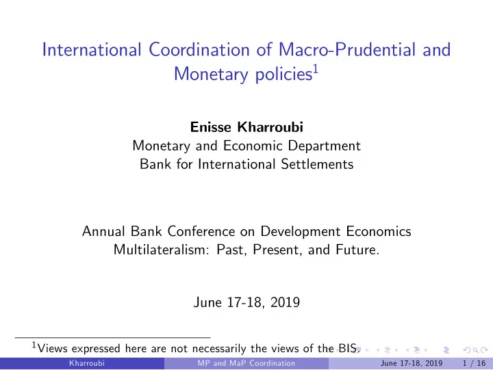
International Coordination of Macro-Prudential and Monetary policies1

Enisse Kharroubi Monetary and Economic Department Bank for International Settlements Annual Bank Conference on Development Economics Multilateralism: Past, Present, and Future. June 17-18, 2019

1Views expressed here are not necessarily the views of the BIS.

Kharroubi () MP and MaP Coordination June 17-18, 2019 1 / 16

Introduction

When is international policy coordination desirable? Literature starting from Obsfeld and Rogo¤ (1992) …nds little gains to international coordination on monetary policy (MP).

I Negligible welfare losses to domestically oriented monetary policies

But what about macro-prudential policy (MaP) ?

I Does a similar kind of result hold ? I What drives cooperation gains ? I How the conduct of other policies (MP) a¤ects these gains? Kharroubi () MP and MaP Coordination June 17-18, 2019 2 / 16

An overview of the main results

Main results

Kharroubi () MP and MaP Coordination June 17-18, 2019 3 / 16

An overview of the main results

Main results

Does a similar kind of result hold?

I Both MaP and MP coordination yields welfare gains. But unlike MP,

MaP coordination is a Pareto improvement.

I MP takes place ex post, after shock are realized and uncertainty has

unraveled, i.e. once countries have become asymmetric

I MaP takes place ex ante (risk sharing), under the veil of ignorance and

has positive GE spill-overs.

Kharroubi () MP and MaP Coordination June 17-18, 2019 3 / 16

An overview of the main results

Main results

Does a similar kind of result hold?

I Both MaP and MP coordination yields welfare gains. But unlike MP,

MaP coordination is a Pareto improvement.

I MP takes place ex post, after shock are realized and uncertainty has

unraveled, i.e. once countries have become asymmetric

I MaP takes place ex ante (risk sharing), under the veil of ignorance and

has positive GE spill-overs.

What drives gains to policy cooperation ?

I Frictions to cross-border capital ‡ows Kharroubi () MP and MaP Coordination June 17-18, 2019 3 / 16

An overview of the main results

Main results

Does a similar kind of result hold?

I Both MaP and MP coordination yields welfare gains. But unlike MP,

MaP coordination is a Pareto improvement.

I MP takes place ex post, after shock are realized and uncertainty has

unraveled, i.e. once countries have become asymmetric

I MaP takes place ex ante (risk sharing), under the veil of ignorance and

has positive GE spill-overs.

What drives gains to policy cooperation ?

I Frictions to cross-border capital ‡ows

How do policies interact with each other ?

I Welfare gains to MaP cooperation larger under Nash MP. Kharroubi () MP and MaP Coordination June 17-18, 2019 3 / 16

Introduction

Some papers in the literature.

Policy coordination:

I extensive literature on MP coordination (cross-border, cross-policy).

Engel (2016) provides a nice survey.

I Much less on MaP coordination. Jeanne (2014), Bengui (2015) and

Engel (2015)

MP and MaP in open economy:

I Objectives: Benigno (2009), Corsetti et. al. (2011), Faia and Monacelli

(2008), Bengui (2014), Senay and Sutherland (2018).

I E¤ectiveness: Rey (dilemma vs. trilemma), Mendoza (2016) and

Aizenmann et al. (2018).

I Leakages: Aiyar (2012) for the UK, Barroso et al. (2016) for Brazil

Liquidity managment/provision

I Under-insurance and pecuniary externalities (Gromb and Vayanos 2002,

Lorenzoni 2008 or Stein 2012), particularly in open economy context (Caballero and Krishnamurthy 2003 or Jeanne and Korinek 2010, Brunnermeier and Sannikov (2014)).

Kharroubi () MP and MaP Coordination June 17-18, 2019 4 / 16

The model

Framework and technologies.

A 3-period economy à la Holmstrom-Tirole (1998) with 2 regions and risk neutral banks maximizing …nal pro…ts.

Kharroubi () MP and MaP Coordination June 17-18, 2019 5 / 16

The model

Framework and technologies.

A 3-period economy à la Holmstrom-Tirole (1998) with 2 regions and risk neutral banks maximizing …nal pro…ts. At date 0, banks hold unit endowment and invest in risky assets.

I At date 1, risky asset returns 1 in one region and 0 in the other I Regions are symmetric and there is no aggregate uncertainty. Kharroubi () MP and MaP Coordination June 17-18, 2019 5 / 16

The model

Framework and technologies.

A 3-period economy à la Holmstrom-Tirole (1998) with 2 regions and risk neutral banks maximizing …nal pro…ts. At date 0, banks hold unit endowment and invest in risky assets.

I At date 1, risky asset returns 1 in one region and 0 in the other I Regions are symmetric and there is no aggregate uncertainty.

At date 1, once uncertainty is resolved:

I If risky assets pay-o¤: banks can save for a return r (< 1) I If risky assets do not pay-o¤: banks can reinvest with unit return 1. Kharroubi () MP and MaP Coordination June 17-18, 2019 5 / 16

The model

Markets

I Ex ante risk sharing: At date 0, banks can issue claims on their risky

assets and buy claims on the other region’s risky assets.

I Ex post market for liquidity: At date 1, once uncertainty is resolved,

banks can exchange liquidity.

Kharroubi () MP and MaP Coordination June 17-18, 2019 6 / 16

The model

Markets

I Ex ante risk sharing: At date 0, banks can issue claims on their risky

assets and buy claims on the other region’s risky assets.

I Ex post market for liquidity: At date 1, once uncertainty is resolved,

banks can exchange liquidity.

Policies

I Monetary policy sets the return r to savings between date 1 and date

2 (deposit facility).

I Macro-prudential policy sets the max limit on banks’ borrowing at

date 0 (leverage ratio or CFM).

Kharroubi () MP and MaP Coordination June 17-18, 2019 6 / 16

The decentralized equilibrium

The portfolio choice for banks: max

L;L;D [1 + L L R1L] R 2 + [βR 1 L + D R2D]

Kharroubi () MP and MaP Coordination June 17-18, 2019 7 / 16

The decentralized equilibrium

The portfolio choice for banks: max

L;L;D [1 + L L R1L] R 2 + [βR 1 L + D R2D]

s.t. D 1 λ and L m (1 + L L)

Kharroubi () MP and MaP Coordination June 17-18, 2019 7 / 16

The decentralized equilibrium

The portfolio choice for banks: max

L;L;D [1 + L L R1L] R 2 + [βR 1 L + D R2D]

s.t. D 1 λ and L m (1 + L L) Assuming max (r; r ) (R2; R

2 ) 1, the equillibrium on market ex

post funding: 1 + L L | {z }

Funding Supply

= βR

1 L + D

| {z }

Funding Demand

Kharroubi () MP and MaP Coordination June 17-18, 2019 7 / 16

The decentralized equilibrium

At the equilibrium, borrowing and issuance constraints bind: D = 1 λ D = 1 λ and L = m (1 + L L) L = m (1 + L L) Negative spill-over: Higher issuance by one region implies lower issuance by the other region.

Kharroubi () MP and MaP Coordination June 17-18, 2019 8 / 16

The decentralized equilibrium

At the equilibrium, borrowing and issuance constraints bind: D = 1 λ D = 1 λ and L = m (1 + L L) L = m (1 + L L) Negative spill-over: Higher issuance by one region implies lower issuance by the other region. At the equilibrium, ex post funding is in excess supply: (R2; R

2 ) = max (r; r ) and

L λ + (1 max (r; r )) L L λ + (1 max (r; r )) L Positive spill-over: Higher issuance by one region allows for larger issuance by the other region.

Kharroubi () MP and MaP Coordination June 17-18, 2019 8 / 16

Optimal monetary policy

The non-cooperative equilibrium

Optimal monetary policy: max

r

π = h 1 +

• 1 1

βR2

• L

i R

2 + (1 R2) (1 λ)

s.t. R2 = R

2 = max (r; r )

Kharroubi () MP and MaP Coordination June 17-18, 2019 9 / 16

Optimal monetary policy

The non-cooperative equilibrium

Optimal monetary policy: max

r

π = h 1 +

• 1 1

βR2

• L

i R

2 + (1 R2) (1 λ)

s.t. R2 = R

2 = max (r; r )

Optimal interest rates in Nash equilibrium: r = r = rn (L; L) β 2

• 1 + max

λ L ; λ L

• Equilibrium interest rate main properties:

I optimal for one region (core), too high for the other (periphery) I decreases in domestic banks leverage. Kharroubi () MP and MaP Coordination June 17-18, 2019 9 / 16

Optimal macro-prudential policy

The non-cooperative equilibrium: Core vs. Periphery

Macro-prudential policy in the core region: max

m

π = h λ +

• 1 1

βrn (L)

• L

i rn (L) s.t. L = m (1 + L L) and L λ + (1 rn (L)) L No trade-o¤ for MaP: higher m ) higher L ) higher pro…ts π

Kharroubi () MP and MaP Coordination June 17-18, 2019 10 / 16

Optimal macro-prudential policy

The non-cooperative equilibrium: Core vs. Periphery

Macro-prudential policy in the core region: max

m

π = h λ +

• 1 1

βrn (L)

• L

i rn (L) s.t. L = m (1 + L L) and L λ + (1 rn (L)) L No trade-o¤ for MaP: higher m ) higher L ) higher pro…ts π Macro-prudential policy in the periphery region: max

m

π = h λ +

• 1 1

βrn (L)

• Li

rn (L) s.t. L = m (1 + L L) L = m (1 + L L) and L λ + (1 rn (L)) L Trade-o¤ for MaP: higher m ) higher L but higher rn (L)

Kharroubi () MP and MaP Coordination June 17-18, 2019 10 / 16

Optimal macro-prudential policy

The non-cooperative equilibrium: Core vs. Periphery

Macro-prudential policy in the core region: max

m

π = h λ +

• 1 1

βrn (L)

• L

i rn (L) s.t. L = m (1 + L L) and L λ + (1 rn (L)) L No trade-o¤ for MaP: higher m ) higher L ) higher pro…ts π Macro-prudential policy in the periphery region: max

m

π = h λ +

• 1 1

βrn (L)

• Li

rn (L) s.t. L = m (1 + L L) L = m (1 + L L) and L λ + (1 rn (L)) L Trade-o¤ for MaP: higher m ) higher L but higher rn (L) Optimal macro-prudential policy in Nash equilibrium: L = λ + (1 rn (L)) L and L = Ln (L)

Kharroubi () MP and MaP Coordination June 17-18, 2019 10 / 16

Optimal macro-prudential policy

The cooperative equilibrium

Cooperative macro-prudential policy: max

m;m

π + π = h λ + λ +

• 1 1

βrn (L)

• (L + L)

i rn (L) s.t. ( L = m (1 + L L) and L = m (1 + L L) L λ + (1 rn (L)) L and L λ + (1 rn (L)) L

Kharroubi () MP and MaP Coordination June 17-18, 2019 11 / 16

Optimal macro-prudential policy

The cooperative equilibrium

Cooperative macro-prudential policy: max

m;m

π + π = h λ + λ +

• 1 1

βrn (L)

• (L + L)

i rn (L) s.t. ( L = m (1 + L L) and L = m (1 + L L) L λ + (1 rn (L)) L and L λ + (1 rn (L)) L No trade-o¤ for core: higher m ) larger global leverage L + L ) larger global pro…ts π + π L = λ + (1 rn (L)) L No trade-o¤ for periphery: higher m ) larger L and hence larger L (positive GE spill-over): L = λ + (1 rn (L)) L

Kharroubi () MP and MaP Coordination June 17-18, 2019 11 / 16

Optimal macro-prudential policy

Comparing Nash and cooperation

In Nash, periphery limits bank leverage to steer FC set in the core. In Coop, periphery internalizes the positive spill-over in bank leverage.

I Gross cross border positions (L; L) are larger I Global funding cost rn (L) is lower Kharroubi () MP and MaP Coordination June 17-18, 2019 12 / 16

Quantifying welfare gains

We consider three parameters of the model

I Cost on cross-border capital ‡ows ( β from 55% to 95%) I Gross foreign liabilities in Core (λ from 40% to 80%) I Gross foreign liabilities in Periphery (λ 0% to 40%)

Global welfare gains distribution (cooperative vs. Nash MP & MaP)

.2 .4 .6 .8 1 2 3 4 5

Note: Welfare gains computed as the ratio of global welfare under cooperative monetary and macro- prudential policies to global welfare under Nash monetary and macro-prudential policies.

in percent

Distribution of global welfare gains

Kharroubi () MP and MaP Coordination June 17-18, 2019 13 / 16

Quantifying welfare gains

Splitting welfare gains by region, by policy

Kharroubi () MP and MaP Coordination June 17-18, 2019 14 / 16

Quantifying welfare gains

Which region bene…ts from coordinating what policies?

Kharroubi () MP and MaP Coordination June 17-18, 2019 15 / 16

Conclusions

We have developed a model of monetary and macro-prudential policy cross-border coordination where

I macro-prudential policy determines bank ex ante leverage. I monetary policy determines the cost of ex post borrowing

Global interest rate under Nash MP is optimal for one region and too high for the other. This creates incentives for periphery to use MaP to a¤ect funding conditions. Trade-o¤: allowing more borrowing vs. correcting ine¢cient funding

• conditions. Main issue: misses the cross-border leverage externality.

Numerically, coordination gains can be sizeable, particurlarly for the

• periphery. Asymmetry matters.

Kharroubi () MP and MaP Coordination June 17-18, 2019 16 / 16