Interactions If a model contains terms u U + v V then UV - PowerPoint PPT Presentation
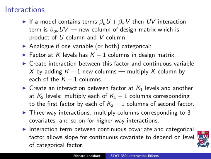
Interactions If a model contains terms u U + v V then UV interaction term is uv UV new column of design matrix which is product of U column and V column. Analogue if one variable (or both) categorical: Factor at K levels has
Interactions ◮ If a model contains terms β u U + β v V then UV interaction term is β uv UV — new column of design matrix which is product of U column and V column. ◮ Analogue if one variable (or both) categorical: ◮ Factor at K levels has K − 1 columns in design matrix. ◮ Create interaction between this factor and continuous variable X by adding K − 1 new columns — multiply X column by each of the K − 1 columns. ◮ Create an interaction between factor at K 1 levels and another at K 2 levels: multiply each of K 1 − 1 columns corresponding to the first factor by each of K 2 − 1 columns of second factor. ◮ Three way interactions: multiply columns corresponding to 3 covariates, and so on for higher way interactions. ◮ Interaction term between continuous covariate and categorical factor allows slope for continuous covariate to depend on level of categorical factor. Richard Lockhart STAT 350: Interaction Effects
Examples: Two way analysis of variance ◮ Experiment involving 2 diets, 3 drugs and 2 experimental units per combination – a factorial experiment. ◮ Y i , j , k is response for Diet i , Drug j and replicate k . ◮ Additive model is Y i , j , k = µ + α i + β j + ǫ i , j , k ◮ Impose restriction α 1 + α 2 = β 1 + β 2 + β 3 = 0. Richard Lockhart STAT 350: Interaction Effects
DESIGN MATRIX 1 1 1 0 1 1 1 0 1 1 0 1 1 1 0 1 1 1 − 1 − 1 1 1 − 1 − 1 X a = 1 − 1 1 0 1 − 1 1 0 1 − 1 0 1 1 − 1 0 1 1 − 1 − 1 − 1 1 − 1 − 1 − 1 ◮ First column corresponds to µ , the grand mean. Second column to α 1 and uses α 2 = − α 1 . Third and fourth columns for β 1 and β 2 use β 3 = − β 1 − β 2 . Richard Lockhart STAT 350: Interaction Effects
◮ Interaction: multiply column 2 by 3 and 2 by 4 to get 1 1 1 0 1 0 1 1 1 0 1 0 1 1 0 1 0 1 1 1 0 1 0 1 1 1 − 1 − 1 − 1 − 1 1 1 − 1 − 1 − 1 − 1 X b = 1 − 1 1 0 − 1 0 1 − 1 1 0 − 1 0 1 − 1 0 1 0 − 1 1 − 1 0 1 0 − 1 1 − 1 − 1 − 1 1 1 1 − 1 − 1 − 1 1 1 ◮ This design matrix corresponds to a model equation Y i , j , k = µ + α i + β j + λ i , j + ǫ i , j , k ◮ Here λ i , j are interaction effects satisfying � i λ i , j = � j λ i , j = 0. Richard Lockhart STAT 350: Interaction Effects
Analysis of Covariance: ANACOVA ◮ Name given to analysis of models in which there are categorical factors and continuous covariates. ◮ In car example: categorical factor VEHICLE, continuous covariate MILEAGE. ◮ Earlier I gave the design matrix for the model in which there are different intercepts for the two cars but 1 common slope. ◮ Thus this model is 2 parallel lines. Richard Lockhart STAT 350: Interaction Effects
◮ Use corner point coding and fit a model in which VEHICLE and MILEAGE interact. ◮ Design matrix for the small data set above is 1 0 0 0 1 0 1000 0 1 0 2000 0 1 1 0 0 1 1 1100 1100 ◮ Last column is the product of columns 2 and 3. ◮ Design matrix corresponds to a model equation with some slope β 1 for the first vehicle and a slope β 1 + γ 2 for the second vehicle. ◮ That is, coefficient of the last column of the design matrix is difference in slopes between the 2 vehicles. Richard Lockhart STAT 350: Interaction Effects
◮ Use of the alternative coding based on an average intercept leads now to the design matrix 1 1 0 0 1 1 1000 1000 1 1 2000 2000 − 3 1 0 0 2 − 3 1 1100 − 1650 2 ◮ Again last column is product of columns 2 and 3. ◮ Coefficient of column 3 is average slope. ◮ Coefficient of last column is difference between slope for vehicle 1 and average slope. ◮ You saw, in assignment 3, how to test the hypothesis of no interaction in this model. Richard Lockhart STAT 350: Interaction Effects
Analysis of Models with Interaction Terms ◮ Usually: use F -tests to try to eliminate higher order interactions (i.e., interactions involving several variables). ◮ Then test for lower order interactions. ◮ To use SAS: put interaction terms in last. Use Type I or sequential SS. ◮ Do not consider models involving a two factor interaction unless individual (also called main ) effects included. ◮ Similarly SS for 3 factor interaction normally adjusted for ◮ all 3 main effects ◮ all 3 two variable interactions of the 3 variables. Richard Lockhart STAT 350: Interaction Effects
Examples Two way ANOVA: influence of SCHOOL, REGION on STAY proc glm data=scenic; class school region ; model Stay = School | Region / E SOLUTION SS1 SS2 SS3 SS4 XPX INVERSE; output out=scout P=Fitted PRESS=PRESS H=HAT RSTUDENT =EXTST R=RESID DFFITS=DFFITS COOKD=COOKD; run ; proc means data=scout; var stay; class school region; run; proc print data=scout; Richard Lockhart STAT 350: Interaction Effects
EDITED SAS OUTPUT The X’X Matrix INTERCEPT SCHOOL 1 SCHOOL 2 REGION 1 REGION 2 INTERCEPT 113 17 96 28 32 SCHOOL 1 17 17 0 5 7 SCHOOL 2 96 0 96 23 25 REGION 1 28 5 23 28 0 REGION 2 32 7 25 0 32 REGION 3 37 3 34 0 0 REGION 4 16 2 14 0 0 DUMMY001 5 5 0 5 0 DUMMY002 7 7 0 0 7 DUMMY003 3 3 0 0 0 DUMMY004 2 2 0 0 0 DUMMY005 23 0 23 23 0 DUMMY006 25 0 25 0 25 DUMMY007 34 0 34 0 0 DUMMY008 14 0 14 0 0 STAY 1090.26 186.85 903.41 310.49 309.87 Richard Lockhart STAT 350: Interaction Effects
EDITED SAS OUTPUT X’X Generalized Inverse (g2) INTERCEPT SCHOOL 1 SCHOOL 2 REGION 1 REGION 2 INTERCEPT 0.0714285714 -0.071428571 0 -0.071428571 -0.071428571 SCHOOL 1 -0.071428571 0.5714285714 0 0.0714285714 0.0714285714 SCHOOL 2 0 0 0 0 0 REGION 1 -0.071428571 0.0714285714 0 0.1149068323 0.0714285714 REGION 2 -0.071428571 0.0714285714 0 0.0714285714 0.1114285714 REGION 3 -0.071428571 0.0714285714 0 0.0714285714 0.0714285714 REGION 4 0 0 0 0 0 DUMMY001 0.0714285714 -0.571428571 0 -0.114906832 -0.071428571 DUMMY002 0.0714285714 -0.571428571 0 -0.071428571 -0.111428571 DUMMY003 0.0714285714 -0.571428571 0 -0.071428571 -0.071428571 DUMMY004 0 0 0 0 0 DUMMY005 0 0 0 0 0 DUMMY006 0 0 0 0 0 DUMMY007 0 0 0 0 0 DUMMY008 0 0 0 0 0 STAY 7.89 1.79 0 2.9304347826 1.5372 Richard Lockhart STAT 350: Interaction Effects
EDITED SAS OUTPUT Dependent Variable: STAY Sum of Mean Source DF Squares Square F Value Pr > F Model 7 132.06558693 18.86651242 7.15 0.0001 Error 105 277.14479360 2.63947422 Corrected Total 112 409.21038053 R-Square C.V. Root MSE STAY Mean 0.322733 16.83864 1.6246459 9.6483186 Source DF Type I SS Mean Square F Value Pr > F SCHOOL 1 36.08413010 36.08413010 13.67 0.0003 REGION 3 95.36410217 31.78803406 12.04 0.0001 SCHOOL*REGION 3 0.61735466 0.20578489 0.08 0.9718 Source DF Type II SS Mean Square F Value Pr > F SCHOOL 1 27.89404890 27.89404890 10.57 0.0015 REGION 3 95.36410217 31.78803406 12.04 0.0001 SCHOOL*REGION 3 0.61735466 0.20578489 0.08 0.9718 Source DF Type III SS Mean Square F Value Pr > F SCHOOL 1 26.05955792 26.05955792 9.87 0.0022 REGION 3 47.01938029 15.67312676 5.94 0.0009 SCHOOL*REGION 3 0.61735466 0.20578489 0.08 0.9718 Source DF Type IV SS Mean Square F Value Pr > F SCHOOL 1 26.05955792 26.05955792 9.87 0.0022 REGION 3 47.01938029 15.67312676 5.94 0.0009 SCHOOL*REGION 3 0.61735466 0.20578489 0.08 0.9718 Richard Lockhart STAT 350: Interaction Effects
EDITED SAS OUTPUT T for H0: Pr > |T| Std Error of Parameter Estimate Parameter=0 Estimate INTERCEPT 7.890000000 B 18.17 0.0001 0.43420487 SCHOOL 1 1.790000000 B 1.46 0.1480 1.22811685 2 0.000000000 B . . . REGION 1 2.930434783 B 5.32 0.0001 0.55072100 2 1.537200000 B 2.83 0.0055 0.54232171 3 1.180588235 B 2.29 0.0241 0.51591227 4 0.000000000 B . . . SCHOOL*REGION 1 1 -0.286434783 B -0.20 0.8455 1.46660342 1 2 -0.618628571 B -0.44 0.6620 1.41099883 1 3 -0.300588235 B -0.19 0.8486 1.57026346 1 4 0.000000000 B . . . SCHOOL*REGION 2 1 0.000000000 B . . . 2 2 0.000000000 B . . . 2 3 0.000000000 B . . . 2 4 0.000000000 B . . . Richard Lockhart STAT 350: Interaction Effects
EDITED SAS OUTPUT NOTE: The X’X matrix has been found to be singular and a generalized inverse was used to solve the normal equations. Estimates followed by the letter ’B’ are biased, and are not unique estimators of the parameters. SCHOOL REGION N Obs N Mean Std Dev Minimum -------------------------------------------------------------------------------- 1 1 5 5 12.3240000 3.3527198 9.7800000 2 7 7 10.5985714 1.1317454 8.2800000 3 3 3 10.5600000 0.7362744 10.1200000 4 2 2 9.6800000 0.6788225 9.2000000 2 1 23 23 10.8204348 2.5061460 8.0300000 2 25 25 9.4272000 1.0978635 7.3900000 3 34 34 9.0705882 1.1911516 7.0800000 4 14 14 7.8900000 0.8332420 6.7000000 -------------------------------------------------------------------------------- Richard Lockhart STAT 350: Interaction Effects
Recommend
More recommend
Explore More Topics
Stay informed with curated content and fresh updates.
