Infotheory for Statistics and Learning Lecture 4 Binary hypothesis - PDF document

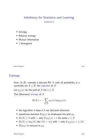
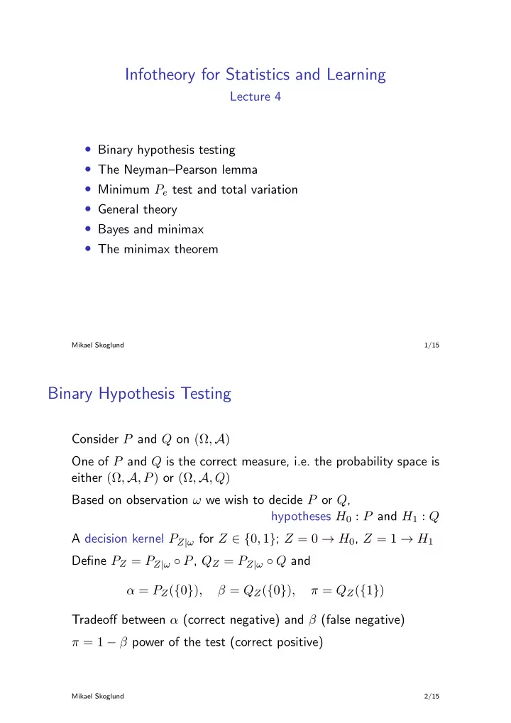
Infotheory for Statistics and Learning Lecture 4 • Binary hypothesis testing • The Neyman–Pearson lemma • Minimum P e test and total variation • General theory • Bayes and minimax • The minimax theorem Mikael Skoglund 1/15 Binary Hypothesis Testing Consider P and Q on (Ω , A ) One of P and Q is the correct measure, i.e. the probability space is either (Ω , A , P ) or (Ω , A , Q ) Based on observation ω we wish to decide P or Q , hypotheses H 0 : P and H 1 : Q A decision kernel P Z | ω for Z ∈ { 0 , 1 } ; Z = 0 → H 0 , Z = 1 → H 1 Define P Z = P Z | ω ◦ P , Q Z = P Z | ω ◦ Q and α = P Z ( { 0 } ) , β = Q Z ( { 0 } ) , π = Q Z ( { 1 } ) Tradeoff between α (correct negative) and β (false negative) π = 1 − β power of the test (correct positive) Mikael Skoglund 2/15

Define β α ( P, Q ) = P Z | ω : P Z ( { 0 } ) ≥ α Q Z ( { 0 } ) inf and � R ( P, Q ) = { ( α, β ) } P Z | ω Mikael Skoglund 3/15 Bounds on R ( P, Q ) Binary divergence for 0 ≤ x ≤ 1 , 0 ≤ y ≤ 1 , d ( x � y ) = x log x y + (1 − x ) log 1 − x 1 − y Then if ( α, β ) ∈ R ( P, Q ) d ( α � β ) ≤ D ( P � Q ) , d ( β � α ) ≤ D ( Q � P ) Also, for all γ > 0 and ( α, β ) ∈ R ( P, Q ) �� log dP �� α − γβ ≤ P dQ > log γ β − α �� log dP �� γ ≤ Q dQ < log γ Mikael Skoglund 4/15

Neyman–Pearson Lemma Define the log-likelihood ratio (LLR), L ( ω ) = log dP dQ ( ω ) For any α , β α ( P, Q ) is achieved by the LLR test  1 L ( ω ) > τ   P Z | ω ( { 0 }| ω ) = λ L ( ω ) = τ  0 L ( ω ) < τ  where τ and λ ∈ [0 , 1] solve α = P ( { L > τ } ) + λP ( { L = τ } ) uniquely Mikael Skoglund 5/15 ⇒ L ( ω ) is a sufficient statistic for { H i } ⇒ R ( P, Q ) is closed and convex, and R ( P, Q ) = { ( α, β ) : β α ( P, Q ) ≤ β ≤ 1 − β 1 − α ( P, Q ) } We have implicitly assumed P ≪ Q (and Q ≪ P ), if this is not the case we can define F = ∪{ A ∈ A : Q ( A ) = 0 while P ( A ) > 0 } Then set P Z | ω ( { 0 }| ω ) = 1 on F and use the LLR test on F c In the extreme P ( F ) = 1 we can set P Z | ω ( { 0 }| ω ) = 1 on F and P Z | ω ( { 0 }| ω ) = 0 on F c , to get α = P ( F ) = 1 and β = Q ( F ) = 0 the test is singular, P ⊥ Q Mikael Skoglund 6/15

With probabilities on { H i } : Pr( H 1 true ) = p , Pr( H 0 true ) = 1 − p Let g ( ω ) = P Z | ω ( { 0 }| ω ) , then the average probability of error � � � � P e = (1 − p ) 1 − g ( ω ) dP + p g ( ω ) dQ � � p − (1 − p ) dP � = g ( ω ) dQ ( ω ) dQ + 1 − p Thus the LLR test is optimal also for minimizing P e , with p τ = log 1 − p and with λ ∈ [0 , 1] arbitrary (e.g. λ = 1 − p ) Mikael Skoglund 7/15 For the total variation between P and Q , we have (per definition) TV ( P, Q ) = sup ( P ( E ) − Q ( E )) E ∈A �� � dP � � = sup dQ ( ω ) − 1 dQ E ∈A E achieved by E = { ω : L ( ω ) > 0 } (if P ≪ Q ) Thus for the LLR test that minimizes P e with p = 1 / 2 ⇒ τ = 0 (and using λ = 0 ), TV ( P, Q ) = P ( { L ( ω ) > 0 } ) − Q ( { L ( ω ) > 0 } ) = α − β α ( P, Q ) = 1 − 2 P e ⇒ P e = (1 − TV ( P, Q )) / 2 For P ⊥ Q , E = F = ∪{ A ∈ A : Q ( A ) = 0 while P ( A ) > 0 } , TV ( P, Q ) = P ( F ) − Q ( F ) = 1 and P e = 0 Mikael Skoglund 8/15

General Decision Theory Given (Ω , A , P ) and assume ( E, E ) is a standard Borel space (i.e., there is a topology T on E , ( E, T ) is Polish, and E = σ ( T ) ) X : Ω → E is measurable if { ω : f ( ω ) ∈ F } ∈ A for all F ∈ E A measurable X is a random • variable if ( E, E ) = ( R , B ) • vector if ( E, E ) = ( R n , B n ) • sequence if ( E, E ) = ( R ∞ , B ∞ ) • object in general Let T be arbitrary, but typically T = R Denote E T = { functions from T to E } , then X is a random • process if ( E, E ) = ( R T , B T ) Mikael Skoglund 9/15 Given (Ω , A , P ) , ( E, E ) and X : Ω → E measurable For a general parameter set Θ let P = { P θ : θ ∈ Θ } be a set of possible distributions for X on ( E, E ) Assume we observe X ∼ P θ (i.e. P θ is the correct distribution), and we are interested in knowing T ( θ ) , for some T : Θ → F A decision rule is a kernel P ˆ T | X = x such that P ˆ T = P ˆ T | X ◦ P X on ( ˆ F, ˆ F ) (for ( ˆ F, ˆ F ) standard Borel, typically ˆ F = F = R and ˆ F = B ) Define a loss function ℓ : F × ˆ F → R and the corresponding risk � �� � R θ ( ˆ ℓ ( T ( θ ) , ˆ dP θ = E θ [ ℓ ( T, ˆ T ) = T ) dP ˆ T )] T | X = x Mikael Skoglund 10/15

Bayes Risk Assume Θ = R and T ( θ ) = θ (for simplicity) Postulate a prior distribution π for θ on ( R , B ) The average risk � � �� � R π (ˆ R θ (ˆ ℓ ( θ, ˆ θ ) = θ ) dπ = θ ) d ( P ˆ θ | X ◦ P θ ) dπ and the Bayes risk R π (ˆ R ∗ π = inf θ ) P ˆ θ | X achieved by the Bayes estimator P ∗ ˆ θ | X = x Mikael Skoglund 11/15 Define P θ | X from π = P θ | X ◦ P θ , then since θ → X → ˆ θ �� �� � � ℓ ( θ, ˆ E π θ ) dP ˆ dP θ θ | X = x � �� �� � � ℓ ( θ, ˆ = θ ) dP ˆ dP θ | X = x dP θ θ | X = x Hence we can define ˆ θ ( x ) via ℓ ( θ, ˆ ℓ ( θ, ˆ � θ ( x )) = θ ) dP ˆ θ | X = x and for each X = x minimize � ℓ ( θ, ˆ θ ( x )) dP θ | X = x ⇒ the Bayes estimator is always deterministic • Thus we can always work with ˆ θ ( x ) instead of P ˆ θ | X • Can also be proved more formally from the fact that R π (ˆ θ ) is linear in P ˆ θ | X and the set { P ˆ θ | X } is convex Mikael Skoglund 12/15

Minimax Risk Let � �� � R ∗ = inf R θ (ˆ ℓ ( θ, ˆ sup θ ) = inf sup θ ) dP ˆ dP θ θ | X = x P ˆ P ˆ θ ∈ Θ θ ∈ Θ θ | X θ | X denote the minimax risk The problem is convex, and we can write R ∗ = inf t s.t. E θ [ ℓ ( θ, ˆ θ )] ≤ t for all θ ∈ Θ θ | X → ˆ over P ˆ θ Mikael Skoglund 13/15 Assume Θ is finite (for simplicity), we get the Lagrangian L (ˆ λ ( θ )( E θ [ ℓ ( θ, ˆ � θ, t, { λ ( θ ) } ) = t + θ )] − t ) θ θ,t L (ˆ and the dual function g ( { λ ( θ ) } ) = inf ˆ θ, t, { λ ( θ ) } ) Note that unless � θ λ ( θ ) = 1 , we get g ( { λ ( θ ) } ) = −∞ Thus sup g ( { λ ( θ ) } ) is attained for λ ( θ ) = a pmf on θ , and � λ ( θ ) E θ [ ℓ ( θ, ˆ π R ∗ sup g ( { λ ( θ ) } ) = sup inf θ )] = sup π ˆ { λ ( θ ) } { λ ( θ ) } θ θ is the worst-case Bayes risk Mikael Skoglund 14/15

Because of weak duality, we always have π R ∗ π ≤ R ∗ sup and strong duality, i.e. R ∗ = sup π R ∗ π holds if • θ is finite and X is finite, or θ ℓ ( θ, ˆ • θ is finite and inf θ, ˆ θ ) > −∞ We have thus established the minimax theorem When strong duality holds the minimax risk is obtained by a deterministic ˆ θ ( x ) Mikael Skoglund 15/15