Individual decision-making under certainty Objects of inquiry Our - PowerPoint PPT Presentation
Introduction Production sets Profit maximization Rationalizability Differentiable case Single-output firms Individual decision-making under certainty Objects of inquiry Our study of microeconomics begins with individual decision-making
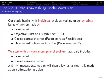
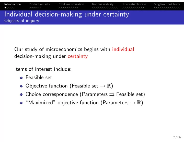
Introduction Production sets Profit maximization Rationalizability Differentiable case Single-output firms Individual decision-making under certainty Objects of inquiry Our study of microeconomics begins with individual decision-making under certainty Items of interest include: Feasible set Objective function (Feasible set → R ) Choice correspondence (Parameters ⇒ Feasible set) “Maximized” objective function (Parameters → R ) 2 / 86
Introduction Production sets Profit maximization Rationalizability Differentiable case Single-output firms Individual decision-making under certainty Course outline We will divide decision-making under certainty into three units: 1 Producer theory Feasible set defined by technology Objective function p · y depends on prices 2 Abstract choice theory Feasible set totally general Objective function may not even exist 3 Consumer theory Feasible set defined by budget constraint and depends on prices Objective function u ( x ) 3 / 86
Introduction Production sets Profit maximization Rationalizability Differentiable case Single-output firms Producer theory: simplifying assumptions Standard model: firms choose production plans (technologically feasible lists of inputs and outputs) to maximize profits Simplifying assumptions include: 1 Firms are price takers (both input and output markets) 2 Technology is exogenously given 3 Firms maximize profits; should be true as long as The firm is competitive There is no uncertainty about profits Managers are perfectly controlled by owners 4 / 86
Introduction Production sets Profit maximization Rationalizability Differentiable case Single-output firms Role of simplifying assumptions No consensus about “correct” view Modeling is an abstraction Relies on simplifying but untrue assumptions Highlight important effects by suppressing other effects Basis for numerical calculations Models can be useful in different ways Relevant predictions reasonably accurate; can sometimes be checked using data or theoretical analysis Failure of relevant predictions can highlight which simplifying assumptions are most relevant “Usual” or “standard” models often fail realism checks; do not skip validation 5 / 86
Introduction Production sets Profit maximization Rationalizability Differentiable case Single-output firms Outline Production sets 1 Profit maximization 2 Rationalizability 3 Rationalizability: the differentiable case 4 Single-output firms 5 6 / 86
Introduction Production sets Profit maximization Rationalizability Differentiable case Single-output firms Outline Production sets 1 Profit maximization 2 Rationalizability 3 Rationalizability: the differentiable case 4 Single-output firms 5 7 / 86
Introduction Production sets Profit maximization Rationalizability Differentiable case Single-output firms Production sets Exogenously given technology applies over n commodities (both inputs and outputs) Definition (production plan) A vector y = ( y 1 , . . . , y n ) ∈ R n where an output has y k > 0 and an input has y k < 0. Definition (production set) Set Y ⊆ R n of feasible production plans; generally assumed to be non-empty and closed. 8 / 86
Introduction Production sets Profit maximization Rationalizability Differentiable case Single-output firms Properties of production sets I Definition (shutdown) 0 ∈ Y . Definition (free disposal) y ∈ Y and y ′ ≤ y imply y ′ ∈ Y . = ⇒ 9 / 86
Introduction Production sets Profit maximization Rationalizability Differentiable case Single-output firms Properties of production sets II Definition (nonincreasing returns to scale) y ∈ Y implies α y ∈ Y for all α ∈ [0 , 1]. Implies shutdown Definition (nondecreasing returns to scale) y ∈ Y implies α y ∈ Y for all α ≥ 1. Along with shutdown, implies π ( p ) = 0 or π ( p ) = + ∞ for all p Definition (constant returns to scale) y ∈ Y implies α y ∈ Y for all α ≥ 0; i.e., nonincreasing and nondecreasing returns to scale. 10 / 86
Introduction Production sets Profit maximization Rationalizability Differentiable case Single-output firms Properties of production sets III Definition (convex production set) y , y ′ ∈ Y imply ty + (1 − t ) y ′ ∈ Y for all t ∈ [0 , 1]. Vaguely “nonincreasing returns to specialization” If 0 ∈ Y , then convexity implies nonincreasing returns to scale Strictly convex iff for t ∈ (0 , 1), the convex combination is in the interior of Y 11 / 86
Introduction Production sets Profit maximization Rationalizability Differentiable case Single-output firms Characterizing Y : Transformation function I Definition (transformation function) Any function T : R n → R with 1 T ( y ) ≤ 0 ⇐ ⇒ y ∈ Y ; and 2 T ( y ) = 0 ⇐ ⇒ y is a boundary point of Y . Can be interpreted as the amount of technical progress required to make y feasible � � The set y : T ( y ) = 0 is the production possibilities frontier (a.k.a. transformation frontier) 12 / 86
Introduction Production sets Profit maximization Rationalizability Differentiable case Single-output firms Characterizing Y : Transformation function II When the transformation function is differentiable, we can define the marginal rate of transformation of good l for good k : Definition (marginal rate of transformation) ∂ T ( y ) ∂ y l MRT l , k ( y ) ≡ , ∂ T ( y ) ∂ y k defined for points where T ( y ) = 0 and ∂ T ( y ) � = 0. ∂ y k Measures the extra amount of good k that can be obtained per unit reduction of good l Equals the slope of the PPF 13 / 86
Introduction Production sets Profit maximization Rationalizability Differentiable case Single-output firms Outline Production sets 1 Profit maximization 2 Rationalizability 3 Rationalizability: the differentiable case 4 Single-output firms 5 14 / 86
Introduction Production sets Profit maximization Rationalizability Differentiable case Single-output firms The Profit Maximization Problem The firm’s optimal production decisions are given by correspondence y : R n ⇒ R n y ( p ) ≡ argmax p · y y ∈ Y � � = y ∈ Y : p · y = π ( p ) Resulting profits are given by profit function π : R n → R ∪ { + ∞} π ( p ) ≡ sup p · y y ∈ Y 15 / 86
Introduction Production sets Profit maximization Rationalizability Differentiable case Single-output firms A note on maxima and suprema We have a tendency to be fast and loose with these, but recall that: A maximum is the highest achieved value A supremum is a least upper bound (which may or may not be achieved) Fact We have not made sufficient assumptions to ensure that a maximum profit is achieved (i.e., y ( p ) � = ∅ ), and so the sup cannot necessarily be replaced with a max . In particular we allow for the possibility that π ( p ) = + ∞ , which can happen if Y is unbounded. 16 / 86
Introduction Production sets Profit maximization Rationalizability Differentiable case Single-output firms A note on convex functions Definition (convexity) f : R n → R is convex iff for all x and y ∈ R n , and all λ ∈ [0 , 1], we have � � λ f ( x ) + (1 − λ ) f ( y ) ≥ f λ x + (1 − λ ) y . In the differentiable case, also characterized by any of If f : R → R , then f ′′ ( x ) ≥ 0 for all x Hessian ∇ 2 f ( x ) is a positive semidefinite matrix for all x f ( · ) lies above its tangent hyperplanes; i.e., f ( x ) ≥ f ( y ) + ∇ f ( y ) · ( x − y ) for all x and y 17 / 86
Introduction Production sets Profit maximization Rationalizability Differentiable case Single-output firms Convex function illustration f ( · ) λ f ( x ) + (1 − λ ) f ( y ) f ( λ x + (1 − λ ) y ) λ x + (1 − λ ) y x y 18 / 86
Introduction Production sets Profit maximization Rationalizability Differentiable case Single-output firms Convexity of π ( · ) Theorem π ( · ) is a convex function. Proof. Fix any p 1 , p 2 and let p t ≡ tp 1 + (1 − t ) p 2 for t ∈ [0 , 1]. Then for any y ∈ Y , p t · y = t p 1 · y +(1 − t ) p 2 · y � �� � � �� � ≤ π ( p 1 ) ≤ π ( p 2 ) ≤ t π ( p 1 ) + (1 − t ) π ( p 2 ) . Since this is true for all p t · y , it holds for sup y ∈ Y p t · y = π ( p t ): π ( p t ) ≤ t π ( p 1 ) + (1 − t ) π ( p 2 ) . 19 / 86
Introduction Production sets Profit maximization Rationalizability Differentiable case Single-output firms A note on homogeneous functions Definition (homogeneity) f : R n → R is homogeneous of degree k iff for all x ∈ R n , and all λ > 0, we have f ( λ x ) = λ k f ( x ) . We will overwhelmingly rely on Homogeneity of degree zero: f ( λ x ) = f ( x ) Homogeneity of degree one: f ( λ x ) = λ f ( x ) 20 / 86
Introduction Production sets Profit maximization Rationalizability Differentiable case Single-output firms Euler’s Law I Theorem (Euler’s Law) Suppose f ( · ) is differentiable. Then it is homogeneous of degree k iff p · ∇ f ( p ) = kf ( p ) . Proof. Homogeneous ⇒ p · ∇ f ( p ) = kf ( p ) proved by differentiating f ( λ p ) = λ k f ( p ) with respect to λ , and then setting λ = 1. Homogeneous ⇐ p · ∇ f ( p ) = kf ( p ) may be covered in section. 21 / 86
Recommend
More recommend
Explore More Topics
Stay informed with curated content and fresh updates.
