Lectures 67: Monotone Comparative Statics, with Applications to - PowerPoint PPT Presentation
Lectures 67: Monotone Comparative Statics, with Applications to Producer Theory Alexander Wolitzky MIT 14.121 1 The Plan for this Week Traditional topic to cover after neoclassical consumer theory is neoclassical producer theory : theory of
Lectures 6—7: Monotone Comparative Statics, with Applications to Producer Theory Alexander Wolitzky MIT 14.121 1
The Plan for this Week Traditional topic to cover after neoclassical consumer theory is neoclassical producer theory : theory of profit-maximizing production choices by a firm. These theories are extremely similar. Plan: � Super-fast treatment of neoclassical producer theory. � Spend time covering critical modern tool for economic analysis: monotone comparative statics . � Illustrate MCS with applications to some modern results in producer theory. 2
Neoclassical Producer Theory in One Sentence “Producers are just like consumers, but they maximize profit instead of utility.” We expand on this just slightly, and show how main results of producer theory follow from results from consumer theory. 3
The Profit Maximization Problem (PMP) Choose production plan y ∈ R n from production possibilities set Y ⊆ R n to maximize profit p · y : max p · y y ∈ Y � � Some prices can be negative. Lets us model inputs and outpus symmetrically. � � Inputs have negative prices (firm pays to use them). � � Outputs have positive prices (firm makes money by producing). � � Neoclassical firm is price taker . � � No market power. � � Study of firms with market power is a topic in industrial organization . � � Firm’s objective is profit maximization . � � In reality, firm is organization composed of individuals with different goals. � � 4 Study of internal behavior and organization of firms is topic in organizational economics .
The PMP and the EMP For our purposes, producer theory leaves everything interesting about firm behavior to other areas of economics, and reduces firm’s problem to something isomorphic to consumer’s expenditure minimization problem. PMP is max p · y . y ∈ Y Letting S = { x ∈ R n : u ( x ) ≥ u } , EMP is min p · x . x ∈ S Up to fiipping a sign, PMP the same as EMP. EMP: consumer chooses bundle of goods x to minimize expenditure, subject to x lying in set S . PMP: firm chooses bundle of goods y to minimize net expenditure 5 (maximize net profit), subject to y lying in set Y .
The PMP and the EMP Solution to EMP: Hicksian demand h ( p ) . Value function for EMP: expenditure function e ( p ) . (omitting u because we hold it fixed) Solution to PMP: optimal production plan y ( p ) . Value function for EMP: profit function π ( p ) . Our treatment of producer theory consists of recalling facts about Hicksian demand and expenditure function, and translating into language of optimal production plan and profit function. 6
Properties of Hicksian Demand/Optimal Production Plans Theorem Hicksian demand satisfies: 1. Homogeneity of degree 0 : for all λ > 0 , h ( λ p ) = h ( p ) . 2. Convexity: if S is convex (i.e., if preferences are convex), then h ( p ) is a convex set. 3. Law of demand: for every p , p i ∈ R n , x ∈ h ( p ) , and x i ∈ h ( p i ) , we have ( p i − p ) ( x i − x ) ≤ 0 . Theorem Optimal production plans satisfy: 1. Homogeneity of degree 0 : for all λ > 0 , y ( λ p ) = y ( p ) . 2. Convexity: if Y is convex, then y ( p ) is a convex set. 3. Law of supply: for every p , p i ∈ R n , y ∈ y ( p ) , and i ∈ y ( p i ) , we have ( p i − p ) ( y i − y ) ≥ 0 . y 7
Properties of Expenditure Function/Profit Function Theorem The expenditure function satisfies: 1. Homogeneity of degree 1 : for all λ > 0 , e ( λ p ) = λ e ( p ) . 2. Monotonicity: e is non-decreasing in p. 3. Concavity: e is concave in p. 4. Shephard’s lemma: under mild conditions (see Lectures 2—3), ∂ e is differentiable, and ∂ p i e ( p ) = h i ( p ) . Theorem The profit function satisfies: 1. Homogeneity of degree 1 : for all λ > 0 , π ( λ p ) = λπ ( p ) . 2. Monotonicity: π is non-decreasing in p. 3. Convexity: π is convex in p. 4. Hotelling’s lemma: under mild conditions, π is differentiable, 8 ∂ and ∂ p i π ( p ) = y i ( p ) .
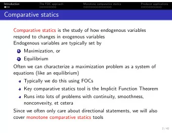
Monotone Comparative Statics: Motivation Comparative statics are statements about how solution to a problem changes with parameters. Core of most applied economic analysis. Last twenty years or so: revolution in how comparative statics are done in economics. Traditional approach: differentiate FOC using implicit function theorem. New approach: monotone comparative statics. 9
Example: Traditional Approach Consider problem: max b ( x , θ ) − c ( x ) x ∈ X � � x is choice variable � � θ is parameter � � b ( x , θ ) is benefit from choosing x given parameter θ � � c is cost of choosing x 10
Example: Traditional Approach max b ( x , θ ) − c ( x ) x ∈ X If X ⊆ R and b and c are differentiable, FOC is ∗ ( θ ) , θ ) = c i ( x ∗ ( θ )) . b x ( x If b and c are twice continuously differentiable and ∗ ( θ ) , θ ) = c ii ( x ∗ ( θ )) , implicit function theorem implies b xx ( x ∗ ( θ ) is continuously differentiable, with derivative that solution x ∗ ( θ ) , θ ) b x θ ( x d ∗ ( θ ) = x . c ii ( x ∗ ( θ )) − b xx ( x ∗ ( θ ) , θ ) d θ If c is convex, b is concave in x , and b x θ > 0, can conclude that ∗ ( θ ) is (locally) increasing in θ . x Intuition: FOC sets marginal benefit equal to marginal cost. If b x θ > 0 and θ increases, then if b is concave in x and c is 11 convex, x must increase to keep the FOC satisfied.
What’s Wrong with This Picture? Unnecessary assumptions: as we’ll see, solution(s) are increasing in θ even if b is not concave , c is not convex , b and c are not differentiable , and choice variable is not continuous or real-valued . Wrong intuition : Intuition coming from the FOC involves concavity of b and convexity of c . This can’t be the right intuition. We’ll see that what’s really needed is an ordinal condition on b – the single-crossing property – which is a more meaningful version of the assumption b x θ > 0. 12
Why Learn Monotone Comparative Statics? Three reasons: 1. Generality: Cut unnecessary convexity and differentiability assumptions. 2. Analytical power: Often, can’t assume convexity and differentiability. (Traditional approach doesn’t work.) 3. Understanding: By focusing on essential assumptions, help to understand workings of economic models. (Don’t get confused about what drives what.) 13
Why Learn Monotone Comparative Statics? Fourth reason: need to understand them to read other people’s papers. � � Costinot, A. “An Elementary Theory of Comparative Advantage.” Econometrica , 2009. [International] � � Acemoglu, D. “When Does Labor Scarcity Encourage Innovation?” Journal of Political Economy , 2010. [Growth/Innovation] � � � Kircher, P. and J. Eeckhout. “Sorting and Decentralized Price Competition.” Econometrica , 2010. [Labor] � � Segal, I. and M. Whinston. “Property Rights.” Chapter for Handbook of Organizational Economics, 2011. [Organizational Econ] � � Acemoglu, D. and A. Wolitzky. “The Economics of Labor Coercion.” Econometrica , 2011. [Political Economy] 14
MCS with 1 Choice Variable and 1 Parameter Start with simple case: X ⊆ R , Θ ⊆ R . Interested in set of solutions X ∗ ( θ ) to optimization problem max f ( x , θ ) x ∈ X Under what conditions on f is X ∗ ( θ ) increasing in θ ? 15
The Strong Set Order What does it mean for set of solutions to be increasing? Relevant order on sets: strong set order . Definition A set A ⊆ R is greater than a set B ⊆ R in the strong set order (SSO) if, for any a ∈ A and b ∈ B , max { a , b } ∈ A , and min { a , b } ∈ B . θ i X ∗ ( θ ) greater than X ∗ i if, whenever x is solution at θ and x is solution at θ i , either 1. x ≥ x i , or 16 2. both x and x i are solutions for both parameters.
Increasing Differences Simple condition on f that guarantees that X ∗ ( θ ) is increasing (in SSO): increasing differences . Definition A function f : R × R → R has increasing differences in ( x , θ ) if, whenever x H ≥ x L and θ H ≥ θ L , we have x , θ H H x , θ H L x , θ L H x , θ L L f − f ≥ f − f . Return to choosing a higher value of x is non-decreasing in θ . Form of complementarity between x and θ . 17
Increasing Differences: Differential Version Theorem If f is twice continuously differentiable, then f has increasing differences in ( x , θ ) iff ∂ 2 f ( x , θ ) ≥ 0 for all x ∈ X , θ ∈ Θ . ∂ x ∂θ Increasing differences generalizes condition on cross-partial derivatives used to sign comparative statics in traditional approach. 18
Topkis’ Monotonicity Theorem Simplest MCS theorem: Theorem (Topkis) If f has increasing differences in ( x , θ ) , then X ∗ ( θ ) is increasing in the strong set order. 19
Back to Example max b ( x , θ ) − c ( x ) x ∈ X If b has increasing differences in ( x , θ ) , then X ∗ ( θ ) is increasing in the strong set order. No assumptions about convexity or differentiability of anything. 20
Necessity Want to find minimal assumptions for given comparative statics result to hold. Is increasing differences minimal assumption? No: increasing differences is cardinal property, but property that X ∗ ( θ ) is increasing is ordinal. What’s ordinal version of increasing differences? 21
Recommend
More recommend
Explore More Topics
Stay informed with curated content and fresh updates.
