(Indicative) outline Introduction Multimedia Indexing and - PowerPoint PPT Presentation

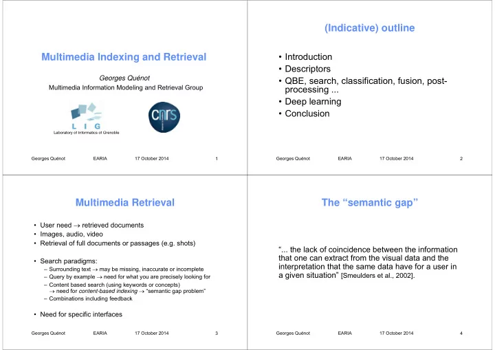
(Indicative) outline • Introduction Multimedia Indexing and Retrieval • Descriptors Georges Quénot • QBE, search, classification, fusion, post- Multimedia Information Modeling and Retrieval Group processing ... • Deep learning • Conclusion Laboratory of Informatics of Grenoble Georges Quénot EARIA 17 October 2014 1 Georges Quénot EARIA 17 October 2014 2 Multimedia Retrieval The “semantic gap” • User need  retrieved documents • Images, audio, video • Retrieval of full documents or passages (e.g. shots) “... the lack of coincidence between the information that one can extract from the visual data and the • Search paradigms: interpretation that the same data have for a user in – Surrounding text  may be missing, inaccurate or incomplete a given situation” [Smeulders et al., 2002] . – Query by example  need for what you are precisely looking for – Content based search (using keywords or concepts)  need for content-based indexing  “semantic gap problem” – Combinations including feedback • Need for specific interfaces Georges Quénot EARIA 17 October 2014 3 Georges Quénot EARIA 17 October 2014 4

The “semantic gap” problem Query BY Example (QBE) Face Query Documents Woman Extraction Extraction Hat Lena Descriptor Descriptors … Matching function Scores (e.g. distance or relevance) ? 122 112 98 85 … Ranking 126 116 102 89 … 131 121 106 95 … 134 125 110 99 … Sorted list … … … … … Georges Quénot EARIA 17 October 2014 5 Georges Quénot EARIA 17 October 2014 6 Example : the QBIC system Content based indexing by supervised learning • Query By Image Content, IBM (stopped demo) Concept annotations Training documents Test documents http://wwwqbic.almaden.ibm.com/cgi-bin/photo-demo Extraction Extraction Descriptors Descriptors Train Model Predict Scores (e.g. probability of concept presence) Georges Quénot EARIA 17 October 2014 7 Georges Quénot EARIA 17 October 2014 8

Descriptors Histograms - general form • Engineered descriptors • A fixed set of disjoint categories (or bins ), numbered from 1 to K . – Color – Texture • A set of observations that fall into these categories – Shape • The histogram is the vector of K values h [ k ] with h [ k ] – Points of interest corresponding to the number of observations that fell into – Motion the category k . – Semantic • By default, the h [ k ] are integer values but they can also – Local versus global be turned into real numbers and normalized so that the h – … vector length is equal to 1 considering either the L 1 or L 2 • Learned descriptors norm – Deep learning • Histograms can be computed for several sets of – Auto encoders observations using the same set of categories producing – … one vector of values for each input set Georges Quénot EARIA 17 October 2014 9 Georges Quénot EARIA 17 October 2014 10 Histograms – text example Image intensity histogram • The set of categories are the possible intensity values • A vector of term frequencies (tf) is an histogram with 8-bit coding, ranging from 0 (black) to 255 (white) or • The categories are the index terms ranges of these intensity values • The observations are the terms in the documents that are also in the index • A tf.idf representation corresponds to a weighting of the bins, less relevant in multimedia since histograms bins are more symmetrical by construction (e.g. built by K-means partitioning) 256-bin 64-bin 16-bin Georges Quénot EARIA 17 October 2014 11 Georges Quénot EARIA 17 October 2014 12

Image color histogram Image color histogram • The set of categories are ranges of possible color values • The set of categories are ranges of possible color values • A common choice is a per component decomposition resulting in a set of parallelepipeds B Representations with the parallelepipeds’ center colors: G 5×5×5-bin 4×4×4-bin 3×3×3-bin 125-bin 27-bin 64-bin R • Any color space can be chosen (YUV, HSV, LAB …) • Any number of bins can be chosen for each dimension • The partition does not need to be in parallelepipeds 5×5×5-bin 3×3×3-bin 4×4×4-bin 125-bin 64-bin 27-bin Georges Quénot EARIA 17 October 2014 13 Georges Quénot EARIA 17 October 2014 14 Image histograms Image histograms • Can be computed on the whole image, • Can be computed by blocks: – One (mono or multidimensional) histogram per image block, – The descriptor is the concatenation of the histograms of the different blocks. – Typically : 4 x 4 complementary blocks but non symmetrical and/or non complementary choices are also possible. For instance: 2 x 2 + full image center • Size problem  only a few bins per dimension or a lot of bins in total Georges Quénot EARIA 17 October 2014 15 Georges Quénot EARIA 17 October 2014 16

Correlograms Fuzzy histograms • Parallelepipeds/bins are taken in the Cartesian product of the color space by itself : six components • Objective: smooth the quantization effect H(r1,g1,b1,r2,g2,b2) (or only four components if the associated to the large size of bins (typically color space is projected on only two dimensions: 4×4×4 for RGB). H(u1,v1,u2,v2)). • Principle: split the accumulated value into two • Bi-color values are taken according to a distribution of adjacent bins according to the distance to the bin the image point couples: centers. – At a given distance one from the other, – And/or in one or more given direction. • Allows for representing relative spatial relationships between colors , • Large data volumes and computations Georges Quénot EARIA 17 October 2014 17 Georges Quénot EARIA 17 October 2014 18 Image normalization Color moments • Objective : to become more robust again illumination • Moments (color distribution global statistics) changes before extracting the descriptors. – Means • Gain and offset normalization: enforce a mean and a – Covariances variance value by applying the same affine transform to all the color components, non-linear variants. – Third order moments • Histogram equalization: enforce an as flat as possible – Can be combined with image coordinates histogram for the luminance component by applying the – Fast and easy to compute and compact same increasing and continuous function to all the color representation but not very accurate components. • Color normalization: enforce a normalization which is similar to the one performed by the human visual: “global” and highly non linear. Georges Quénot EARIA 17 October 2014 19 Georges Quénot EARIA 17 October 2014 20

Texture descriptors Gabor transforms • Computed on the luminance component only • Frequential composition or local variability (Circular) Gabor filter of direction  , of wavelength  and of extension  : • Fourier transforms • Gabor filters • Neuronal filters • Cooccurrence matrices Energy of the image through this filter: • Normalization possible. Georges Quénot EARIA 17 October 2014 21 Georges Quénot EARIA 17 October 2014 22 Gabor transforms Gabor transforms • Circular: Elliptic: Circular: – scale  , angle  , variance  , –  multiple of  , typically :  = 1.25  , (“same number” of wavelength whatever the  value)    • Elliptic:  – scale  , angle  , variances   and   ,    –   and   multiples of  , typically :   = 0.8  et   = 1.6  ,  • 2 independent variables: – scale  : N values (typically 4 to 8) on a logarithmic scale  (typical ratio of  2 to 2)  – angle  : P values (typically 8), – N.P elements in the descriptor, Georges Quénot EARIA 17 October 2014 23 Georges Quénot EARIA 17 October 2014 24