Indexing and Cla In lassify fying Gig igabytes of Time Series - PowerPoint PPT Presentation
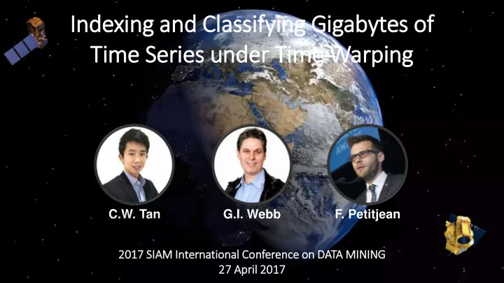
Indexing and Cla In lassify fying Gig igabytes of Time Series under Tim ime Warping C.W. Tan G.I. Webb F. Petitjean 20 2017 17 SIA SIAM In International l Con onference on on DATA MIN INING 27 27 April il 20 2017 17 1 2
Indexing and Cla In lassify fying Gig igabytes of Time Series under Tim ime Warping C.W. Tan G.I. Webb F. Petitjean 20 2017 17 SIA SIAM In International l Con onference on on DATA MIN INING 27 27 April il 20 2017 17 1
2 Footage courtesy of ESA - European Space Agency
Temporal Land-Cover Maps 3
What can we do with it? • Yield forecast 4
What can we do with it? • Yield forecast • Fire spread model 5
What can we do with it? • Yield forecast • Fire spread model • City pollution absorption models • and more… 6
One Im Image is not enough! Impossible to differentiate them! 7
What’s possible? → Temporal Evolution Satellite Image Time Series (SITS) Analysis Petitjean, F., Kurtz, C., Passat, N., & Gançarski, P. Every pixel represents a geographic area (2012). Spatio-temporal reasoning for the classification (Lat, Lon) on Earth of satellite image time series. Pattern Recognition 8 Letters, 33(13), 1805-1815.
How to do this? • Time series classification • State-of-the-art, Nearest Neighbor coupled with Dynamic Time Warping (NN-DTW) [1] • Many phenomena of interest – vegetation cycles, have periodic behavior which can be modulated by weather artifacts. [2] • Too short for the Bag-of-word-type approaches to perform best • Length of 46 – 52 • Less features in the series • BOSS-VS [3] achieved around 40% error rate, NN-DTW achieved 16% [1] Bagnall, A., & Lines, J. (2014). An experimental evaluation of nearest neighbour time series classification. technical report# CMP-C14-01. Department of Computing Sciences , University of East Anglia , Tech. Rep. [2] Petitjean, F., Inglada, J., & Gançarski, P. (2012). Satellite image time series analysis under time warping. IEEE Transactions on Geoscience and Remote Sensing , 50(8), 3081-3095. [3] Schäfer, P. (2016). Scalable time series classification. Data Mining and Knowledge Discovery , 30 (5), 1273-1298. 9
Example series for different crops Corn Wheat Soybean Broad-Leaved Tree 10
Traditionally X 1,000,000 NN Classifier NN 1,000 X 100 1,000 How long 1,000 will it 100 million examples take? 1,000 A million pixels = A million sequences 11
Most research in time series classification 12
Problem Statement • Anytime Time Series Classification • Classify a query at any given time with high accuracy • Without constraints on computational resources at training time • In Nearest Neighbor classification • Find the nearest neighbor much faster than full linear scan • Traditional techniques • Build an indexing structure in Euclidean Space • k- d tree, R tree, LSH … • Does not work with DTW 13
In Indexing with Hierarchical Clusters 14
Time Series In Indexing • Hierarchical K-means indexing structure • Uses a priority search to speedup the Set of time series process [1] • Leverage off a recent work on DTW DBA averaging • DTW Barycenter Averaging (DBA) [2, 3] • [2] shows that K-means and DBA allows Average time series faster and more accurate classification [1] Muja, M., & Lowe, D. G. (2014). Scalable nearest neighbor algorithms for high dimensional data. IEEE Transactions on Pattern Analysis and Machine Intelligence , 36 (11), 2227-2240. [2] Petitjean, F., Forestier, G., Webb, G. I., Nicholson, A. E., Chen, Y., & Keogh, E. (2014, December). Dynamic time warping averaging of time series allows faster and more accurate classification. In Data Mining (ICDM), 2014 IEEE International Conference on (pp. 470-479). IEEE. 15 [3] Petitjean, F., Ketterlin, A., & Gançarski, P. (2011). A global averaging method for dynamic time warping, with applications to clustering. Pattern Recognition , 44 (3), 678-693.
Time Series In Indexing Unexplored Traverse to • At testing time branches to first leaf here SearchTree ( T , Q , K ) Traverse ( T , Q , PQ , Res ) PQ , Res = empty priority queues if ( T is leaf) then Traverse ( T, Q, PQ, Res ) Res.addAll(T.data) with distances to Q while (within contract and PQ not empty) do else nextBranch = PQ . pop () C = T.child nearest to Q Traverse ( nextBranch , Q , PQ, Res ) PQ.addAll ( T.child except C ) with end while distances to Q Traverse ( C , Q , PQ , Res ) return Res . pop ( k ) end if 16
Time Series In Indexing Unexplored Traverse to • At testing time branches to first leaf here SearchTree ( T , Q , K ) Traverse ( T , Q , PQ , Res ) PQ , Res = empty priority queues if ( T is leaf) then Traverse ( T, Q, PQ, Res ) Res.addAll(T.data) with distances to Q while (not stop and PQ not empty) do else nextBranch = PQ . pop () C = T.child nearest to Q Traverse ( nextBranch , Q , PQ, Res ) PQ.addAll ( T.child except C ) with end while distances to Q These are a NN Traverse ( C , Q , PQ , Res ) search with DTW return Res . pop ( k ) end if O(L 2 ) time Apply DTW lower bounds, LB Keogh to minimize DTW computations and have 2 PQ 17
Lower Bound Keogh (L (LB Keogh) 1. Computes Upper ( U ) and Lower ( L ) envelope for query Q 2. Computes the distance of the projection of a candidate sequence C onto the envelope Only need to compute the envelopes for Q once!! [1] Keogh, E. (2002, August). Exact indexing of dynamic time warping. In Proceedings of the http://www.cs.ucr.edu/~eamonn/LB_Keogh.htm 28th international conference on Very Large Data Bases (pp. 406-417). VLDB Endowment. 18
Simple example 19
Time Series In Indexing Example Classes: • Alphabets are Blue Centroids of each Red cluster • Numbers are actual time series in training set • 23 time series in the training set 7 20
Time Series In Indexing Example Query time series Actual NN: 13 7 Target 21
Time Series In Indexing Example Query time series Actual NN: 13 LB Distance to A: 0.895 B: 6.157 C: 0.814 DTW Distance to A: 4.893 7 B: Skip (16.920) C: 5.231 Target LB Priority Queue : {B} Priority Queue Distance to Query : {6.2} DTW Priority Queue : {C} 22 Priority Queue Distance to Query : {5.2}
Time Series In Indexing Example Query time series Actual NN: 13 LB Distance to 6: 20.253 D: 0.573 2: 0.781 DTW Distance to 6: Skip (40.592) 7 D: 6.668 2: 10.194 Target LB Priority Queue : {B, 6} Priority Queue Distance to Query : {6.2, 20.3} DTW Priority Queue : {C, 2} 23 Priority Queue Distance to Query : {5.2, 10.2}
Time Series In Indexing Example Query time series Actual NN: 13 LB Distance to H: 1.252 I: 0.726 19: 1.321 DTW Distance to H: 11.387 7 I: 4.839 19: 9.335 Target LB Priority Queue : {B, 6} Priority Queue Distance to Query : {6.2, 20.3} DTW Priority Queue : {C, 19, H, 2} 24 Priority Queue Distance to Query : {5.2, 9.3, 11.4, 10.2}
Time Series In Indexing Example NN : {18} Distance to Query : 4.911 Query time series Actual NN: 13 LB Distance to 18: 1.097 21: 1.726 DTW Distance to 18: 4.911 7 21: 9.548 Target LB Priority Queue : {B, 6} Priority Queue Distance to Query : {6.2, 20.3} DTW Priority Queue : {C, 19, H, 2} 25 Priority Queue Distance to Query : {5.2, 9.3, 11.4, 10.2}
Time Series In Indexing Example NN : {18} Distance to Query : 4.911 Next to explore Query time series LB Distance of B > DTW Actual NN: 13 Distance of C • Current NN is 18, Class 1 • Not actual NN • Next to explore is Node C • Dequeue C from DTW Priority 7 Queue Target LB Priority Queue : {B, 6} Priority Queue Distance to Query : {6.2, 20.3} DTW Priority Queue : {C, 19, H, 2} 26 Priority Queue Distance to Query : {5.2, 9.3, 11.4, 10.2}
Time Series In Indexing Example NN : {13} Distance to Query : 2.930 Query time series Actual NN: 13 LB Distance to 13: 0.672 F: 0.497 G: 2.585 DTW Distance to 13: 2.930 7 F: 4.249 G: 11.446 Target LB Priority Queue : {B, 6} Priority Queue Distance to Query : {6.2, 20.3} DTW Priority Queue : {F, 19, H, 2, G} 27 Priority Queue Distance to Query : {4.2, 9.3, 11.4, 10.2, 11.4}
Time Series In Indexing Example NN : {13} Distance to Query : 4.249 Next to explore Query time series LB Distance of B > DTW Actual NN: 13 Distance of F • Found NN in 2 tree traversals • Next to explore is Node F • Dequeue F from DTW Priority 7 Queue Target LB Priority Queue : {B, 6} Priority Queue Distance to Query : {6.2, 20.3} DTW Priority Queue : {F, 19, H, 2, G} 28 Priority Queue Distance to Query : {4.2, 9.3, 11.4, 10.2, 11.4}
Comparison with state of the art 29
Experiments • Compared with NN-DTW with LB_Keogh • at x % of the time of the full NN-DTW • 1%, 10%, 20%, 30%, 40%, 50% • Satellite Dataset • Train 1M series • Length 46 • Number of classes: 24 • 84 UCR Repository [1] [1] Chen, Yanping, et al. "The ucr time series classification archive." URL www.cs.ucr.edu/~ eamonn/time_series_data (2015). 30
Results on the satellite data State of the art – random sampling If given only 0.1ms Our approach to classify a pixel, we do better by 22% At 1ms to classify a pixel, we do better by 18% Almost same accuracy as full search but 1,000x faster! • Classifying Houston would take 4 hours instead of 1 year! 31
Recommend
More recommend
Explore More Topics
Stay informed with curated content and fresh updates.


