Independence Assumptions Kostas Tzoumas, Amol Deshpande, Christian - PowerPoint PPT Presentation
Lightweight Graphical Models for Selectivity Estimation Without Independence Assumptions Kostas Tzoumas, Amol Deshpande, Christian S. Jensen Presented by Guozhang Wang DB Lunch, Nov 23rd, 2011 Lightweight Graphical Models for Selectivity
Lightweight Graphical Models for Selectivity Estimation Without Independence Assumptions Kostas Tzoumas, Amol Deshpande, Christian S. Jensen Presented by Guozhang Wang DB Lunch, Nov 23rd, 2011
Lightweight Graphical Models for Selectivity Estimation Without With Little Independence Assumptions Kostas Tzoumas, Amol Deshpande, Christian S. Jensen Presented by Guozhang Wang DB Lunch, Nov 23rd, 2011
Motivation: Query Optimization The “best” join plan ◦ Cost = # intermediate tuples along the path Errors in estimates lead to wrong plan
Selectivity Estimation 𝑀𝑃 = 𝑀 ∗ 𝑃 ∗ 𝑄𝑠 (𝑚. 𝑝𝑠𝑒𝑓𝑠𝑙𝑓𝑧 = 𝑝. 𝑝𝑠𝑒𝑓𝑠𝑙𝑓𝑧 𝑝. 𝑢𝑝𝑢𝑏𝑚𝑞𝑠𝑗𝑑𝑓 𝜗 𝑢1, 𝑢2 𝑚. 𝑓𝑦𝑢𝑓𝑜𝑒𝑓𝑒𝑞𝑠𝑗𝑑𝑓𝜗 𝑓1, 𝑓2 ) Equal to distribution estimation ◦ Estimation based on histograms ◦ How complicated histograms we need?
Correlations Matter in Estimation Need multi-dim. histograms to capture correlation between attributes
Idea # 1 : Full Independence Assume attributes are mutually indept. ◦ Only need 1-D histograms, one for each attribute Estimates done by multiplication 𝑄𝑠 𝑚. 𝑝𝑙 = 𝑝. 𝑝𝑙 𝑝. 𝑢𝑞 𝜗 𝑢1, 𝑢2 𝑚. 𝑓𝑞𝜗 𝑓1, 𝑓2 = 𝑄𝑠 𝑚. 𝑝𝑙 = 𝑝. 𝑝𝑙 * 𝑄𝑠 𝑝. 𝑢𝑞𝜗 𝑢1, 𝑢2 * 𝑄𝑠 𝑚. 𝑓𝑞𝜗 𝑓1, 𝑓2 Possible Big Error!
Idea # 2 : No Independence Any subsets of attributes could be correlated ◦ Construct one n-Dim histogram, n = # total attributes in the database Estimates done by marginalization 𝑄𝑠 𝑚. 𝑝𝑙 = 𝑝. 𝑝𝑙 𝑝. 𝑢𝑞 𝜗 𝑢1, 𝑢2 𝑚. 𝑓𝑞𝜗 𝑓1, 𝑓2 = 𝑄𝑠 (. . ) !𝑚.𝑝𝑙… Storage Blowup!
Idea # 3 : Cond. Independence [SIGMOD’01] Capture correlation in a Bayes network ◦ BN model is constructed at start ◦ Estimates done by computing joint dist’n Query Q Model Database Constructor Selectivity Size(Q) Estimator offline execution time
Bayesian Network Each node x has a conditional probability distribution P( x |Pa( x )) Encodes independence in directed graph P(R|S, G ) S G Sunny Day Good Lunch t t 0.8 0.2 t f 0.6 0.4 f t 0.2 0.8 Ride to Work f f 0.01 0.99 Job Done Happy
BN Construct Nodes ◦ Each attribute: a ◦ Each foreign key: join indicator J f Edges ◦ Find the model that maximize log-likelihood given data (greedy local structure search) ◦ Parameters estimation after the structure is decided
Selectivity Estimation in BN Extend the query to include all the involved nodes’ parents Multiplication along the graph to get the joint distribution select * from P , S where P.Strain = Strain-ID ..
Cons. of BN Model is still too complicated… ◦ Construction is expensive ◦ Selectivity estimation is expensive Query Q Model Database Constructor Selectivity Size(Q) Estimator offline execution time
The Tradeoff Spectrum Full No Independence Independence Cond. ? Independence Red: better efficiency, worse accuracy Blue: better accuracy, worse efficiency
Idea # 4 : Constraint BN Dep. Further restrict the structure of BN: ◦ Acyclic [SIGMOD’01] ◦ Fixed structure [this paper] Challenge: how to choose the fixed structure to get the good tradeoff in the spectrum? ◦ Model simple enough for efficient algorithms ◦ Model still capture important correlations
Fixed Structure BN Within a table ◦ Attributes have at most one parent: tree structure Across a table ◦ Joint indicators have at most two parents ◦ No other cross-table edges 3D histograms only, scalable construction
Fixed Structure BN Construct Nodes ◦ Each attribute a ◦ sssssssssssssssssssssssssssssssssssssssssssssssss ◦ Each join indicator J f ssssssssssssssssssssssssss based on workload Edges ◦ Within a table: maximum spanning tree ◦ Across tables: best parent from each table ◦ Weights based on mutual information
Selectivity Est. in Fixed BN Transform BN into a junction tree ◦ Moralization
Selectivity Est. in Fixed BN Transform BN into a junction tree
Selectivity Est. in Fixed BN Transform BN into a junction tree
Selectivity Est. in Fixed BN Transform BN into a junction tree
Selectivity Est. in Fixed BN Extract the subtree related to the query select c_name, c_address from lineitem,orders,customer where l_orderkey=o_orderkey and o_custkey=c_custkey and l_sdate <=“25/7/2011” and c_acctbal<=200000
Selectivity Est. in Fixed BN Tree algorithms for joint distribution ◦ Sum-product ◦ DP select c_name, c_address from lineitem,orders,customer where l_orderkey=o_orderkey and o_custkey=c_custkey and l_sdate <=“25/7/2011” and c_acctbal<=200000
Experiments Implementation ◦ Model construction outside DBMS, use queries to get distributions ◦ Stores junction tree as tables in catalog ◦ Replace selectivity estimation procedure Compare with PostgresSQL
Efficiency and Accuracy Execution & optimization times Cost of plans (intermediate tuples)
Scalability Error: max(real,estimate) / min(real,estimate)
Conclusion Thank Y hank You! ou! Inaccurate selectivity estimation leads to bad plan Fixed structure BN is a good tradeoff between efficiency and accuracy (?)
Recommend
More recommend
Explore More Topics
Stay informed with curated content and fresh updates.
