Independence and Conditional Probability August 5, 2019 August 5, - PowerPoint PPT Presentation
Independence and Conditional Probability August 5, 2019 August 5, 2019 1 / 79 Midterm The Midterm is next week Tuesday, August 13. Approximately 50 multiple choice questions. You do not need a scantron. Questions will be mostly conceptual.
Independence and Conditional Probability August 5, 2019 August 5, 2019 1 / 79
Midterm The Midterm is next week Tuesday, August 13. Approximately 50 multiple choice questions. You do not need a scantron. Questions will be mostly conceptual. You may bring any basic or graphing calculator. I will bring extra scratch paper. Section 3.1 August 5, 2019 2 / 79
Extra Credit Opportunity Write an exam question that would be appropriate for your midterm. The midterm will cover material from Chapters 1, 2, and 3. Your exam question must come from material covered in class, your homeworks, or your labs. Questions may be either multiple choice or short answer. To receive any credit, you must write an original question and provide both the question and the correct answer. These can be submitted on iLearn (Assignments tab). It opens today at 9:30am and will close on Thursday at 11:59pm. Section 3.1 August 5, 2019 3 / 79
Independence Independence of random processes is similar to independence of variables and observations. We say that two random processes are independent if knowing the outcome of one provides no useful information about the outcome of the other. Section 3.1 August 5, 2019 4 / 79
Independence For example, consider our discussion on rolling 2 six-sided dice. The roll of the first die has no effect on the roll of the second die. Thus our two dice rolls are independent of one another. Section 3.1 August 5, 2019 5 / 79
Independence We’ve already calculated the probability of the two rolls both being a 1 1/6 of the time the first roll is a 1 A further 1/6 of those times the second is also a 1 . So we decided that the probability was (1 / 6) × (1 / 6) = 1 / 36. Multiplying these probabilities together works because the two events are independent. Section 3.1 August 5, 2019 6 / 79
Multiplication Rule for Independent Processes Let A and B be events from two different and independent processes. Then the probability that both A and B occur can be calculated as the product of their separate probabilities: P ( A and B ) = P ( A ) × P ( B ) Similarly, if there are k events A 1 , . . . , A k from k independent processes, then the probability they all occur is P ( A 1 ) × P ( A 2 ) × · · · × P ( A k ) Section 3.1 August 5, 2019 7 / 79
Example About 9% of people are left-handed. Suppose 2 people are selected at random from the U.S. population. Because the sample size of 2 is very small relative to the population, it is reasonable to assume these two people are independent. 1 What is the probability that both are left-handed? 2 What is the probability that both are right-handed? Section 3.1 August 5, 2019 8 / 79
Example: Both Left-Handed What is the probability that both are left-handed? Let L 1 be the event that the first person is left-handed and L 2 the event that the second person is left-handed. We are told that 9% of people are left-handed, so P ( L 1 ) = P ( L 2 ) = 0 . 09. Section 3.1 August 5, 2019 9 / 79
Example: Both Left-Handed What is the probability that both are left-handed? We are assuming that these people are independent, so we can use the multiplication rule: P ( L 1 and L 2 ) = P ( L 1 ) × P ( L 2 ) = (0 . 09) × (0 . 09) = 0 . 0081 or 0.81% (this is highly unlikely!) Section 3.1 August 5, 2019 10 / 79
Example: Both Right-Handed What is the probability that both are right-handed? First, assume that everyone is either right- or left-handed. Then L c 1 is the event that the first person is right-handed and L c 2 is the event that the second person is right-handed. From the previous slide, we decided that P ( L 1 ) = P ( L 2 ) = 0 . 09 So P ( L c 1 ) = 1 − P ( L 1 ) = 1 − 0 . 09 = 0 . 91 and P ( L c 2 ) = 0 . 91 Section 3.1 August 5, 2019 11 / 79
Example: Both Right-Handed What is the probability that both are right-handed? We are still assuming that these people are independent, so we can again use the multiplication rule: P ( L c 1 and L c 2 ) = P ( L c 1 ) × P ( L c 2 ) = (0 . 91) × (0 . 91) = 0 . 8281 or 82.81%. Section 3.1 August 5, 2019 12 / 79
Disjoint Events - Independent? If two events are disjoint, are they independent? Section 3.1 August 5, 2019 13 / 79
Disjoint Events- Independent? If two events are disjoint, are they independent? Recall that independent events have no relationship with one another. This means that if we know something about event A , we don’t get any information about event B . For disjoint events, if event A occurs, we can be totally certain that event B did not occur. Therefore they are dependent . Section 3.1 August 5, 2019 14 / 79
Example Consider two disjoint events for rolling a six-sided die. Let A = { 1 } be the event that I roll a 1 and B = { 2 } the event that I roll a 2 . If I know that A occurred, then I can be 100% sure that B did not occur. If I know that A did not occur, then I know that the roll must be a 2 , 3 , 4 , 5 , or 6 . Now there are five possible options instead of six! We’ve narrowed down our options, so knowing that I did not roll a 1 has given us some useful information. Therefore A and B can’t be independent. Section 3.1 August 5, 2019 15 / 79
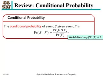
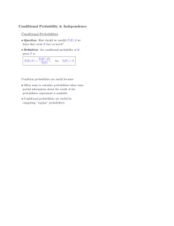
Conditional Probability We can get far more information out of the relationships between multiple variables than we can from a single variable. For example Recall our case study on the malaria vaccine. We can look at P(infection), but that doesn’t tell us anything about the efficacy of the vaccine. Instead, we want to look at the probability that a person develops infection if they were vaccinated . We compare this to the probability that a person develops infection if they were not vaccinated. Section 3.2 August 5, 2019 16 / 79
Contingency Table Probabilities Let’s consider a data set on a machine learning classifier. The classifier is designed to take images and determine whether each one is about fashion. The classifier groups 1822 photos into either ”fashion” or ”not fashion”. Separately, these photos are grouped into ”fashion” and ”not fashion” by a group of people. We take these groupings as the truth that the classifier is trying to get at. Section 3.2 August 5, 2019 17 / 79
Contingency Table Probabilities We can take these groupings and build them into a contingency table. truth Fashion Not Total Fashion 197 22 219 classifier Not 112 1491 1603 Total 309 1513 1822 Section 3.2 August 5, 2019 18 / 79
Contingency Table Probabilities We think about this a lot with classification problems! truth Total fashion not fashion 197 22 219 pred fashion classifier 112 1491 1603 pred not Total 309 1513 1822 When we build our classifier, we want to know the rate at which it correctly and incorrectly identifies fashion and not fashion . This will give us an idea of how successful our classifier is. Is it a good classifier? Should we try a different machine learning algorithm? Section 3.2 August 5, 2019 19 / 79
Example: Contingency Table Probabilities 1 If the photo is actually about fashion, what is the probability that the classifier correctly identified it as being about fashion? 2 If the classifier predicted that a photo was not about fashion, what is the probability that it was incorrect? Section 3.2 August 5, 2019 20 / 79
Example: Contingency Table Probabilities If the photo is actually about fashion, what is the probability that the classifier correctly identified it as being about fashion? truth Total fashion not fashion 197 22 219 pred fashion classifier 112 1491 1603 pred not Total 309 1513 1822 We know that the photo is actually about fashion, so we focus our attention to the column where truth is fashion . Then within this column, we look for the number of times the classifier pred fashion out of the total number of fashion photos. Section 3.2 August 5, 2019 21 / 79
Example: Contingency Table Probabilities If the photo is actually about fashion, what is the probability that the classifier correctly identified it as being about fashion? truth Total fashion not fashion 197 22 219 pred fashion classifier 112 1491 1603 pred not Total 309 1513 1822 P ( classifier is pred fashion given truth is fashion ) = 197 309 or 0.638, a reasonable correct identification rate for fashion. Section 3.2 August 5, 2019 22 / 79
Example: Contingency Table Probabilities If the classifier predicted that a photo was not about fashion, what is the probability that it was incorrect? truth Total fashion not fashion 197 22 219 pred fashion classifier 112 1491 1603 pred not Total 309 1513 1822 We know that classifier is pred not fashion, so we focus our attention to this row. We want to know the probability that it was incorrect, or in truth is fashion . Section 3.2 August 5, 2019 23 / 79
Example: Contingency Table Probabilities If the classifier predicted that a photo was not about fashion, what is the probability that it was incorrect? truth Total fashion not fashion 197 22 219 pred fashion classifier 112 1491 1603 pred not Total 309 1513 1822 P ( truth is fashion given classifier is pred not ) = 112 1603 or 0.070, a low misidentification rate for fashion photos. Section 3.2 August 5, 2019 24 / 79
Recommend
More recommend
Explore More Topics
Stay informed with curated content and fresh updates.
