In Search of a Unifying Theory for Image Interpretation Donald Gem - PowerPoint PPT Presentation

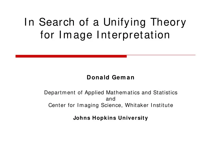
In Search of a Unifying Theory for Image Interpretation Donald Gem an Department of Applied Mathematics and Statistics and Center for Imaging Science, Whitaker Institute Johns Hopkins University

Outline � Semantic Scene Interpretation � Frameworks, Theories � Hierarchical Testing � The Efficiency of Abstraction

Orientation within Imaging � Sensors to Images � Images to Images � Images to Words

Images to Words � Computational vision remains a major challenge (and natural vision a mystery). � Assume one grey-level image. � Generally massive local ambiguity . � But less so globally , e.g., at the semantic level of keywords.

Tasks � Object identification (find my car) and categorization (find all cars) � Recognition of multiple objects, activities, contexts, etc. Ideally, a description machine from images to rich scene interpretations.

Slide credit: Li Fei Fei Scene

Is that a picture of Mao?

Are there cars?

Multiple Object Categorization sky building flag wall face banner street lamp bus bus cars

Scene Categorization

Confounding Factors � Clutter � Invariance to � Viewpoint � Photometry � Variation � Invariance vs. Selectivity

Clutter

Klimt, 1913 Clutter

Slide credit: Li Fei Fei Viewpoint Variation Michelangelo 1475-1564

Slide credit: Shimon Ullman Lighting Variation

Magritte, 1957 Occlusion

Xu, Beihong 1943 Occlusion

Within-Class Variation

Within-Class Variation

How Many Samples are Needed?

Where Things Stand � Reasonable performance for several classes of semi-rigid objects. � Even for face detection, a large “ROC gap” with human vision. � Full scene parsing is currently beyond reach.

Where Are the Faces?

The ROC Gap: Face Detection Current Com puter Vision : Approximately one hallucination per scene at ninety percent detection.

Bruegel, 1564

Francisco’s Kitchen

Notation I : greyscale image : distinguished descriptions of I Y Ex: strings of ( class,pose ) pairs Y ∈ {0} ∪ Y : hidden r.v. Ŷ (I) : estimated description(s) from Y L={(I,Y)} : finite training set, in theory i.i.d. under P(I,Y)

Description Machine Specs � DESIGN and LEARNING: An explicit set of instructions for building Ŷ involving from L . � COMPUTATION: An explicit set of instructions for evaluating Ŷ (I) with as little computation as possible. � ANALYSI S: A “supporting theory” which guides construction and predicts performance

Ground Truth � For Y sufficiently restricted, reasonable to assume a “true interpetation” of I : � Y = { face} , Y = { indoor, outdoor} ,… More generally, Y = {(c 1 , θ 1 ),…, (c k , θ k )} , limited to � specific categories and rough poses. � Corresponds to P emp (Y|I)= δ f(I) (Y) where P emp (I,Y) is the empirical distribution over a gigantic sample (I 1 ,Y 1 ), (I 2 ,Y 2 ),…

Outline � Semantic Scene Interpretation � Frameworks, Theories � Hierarchical Testing � The Efficiency of Abstraction

Deceased Frameworks � Traditional “AI” (60’s, 70’s) � Stepwise, bottom-up 3D metric reconstruction (80’s) � Algebraic, geometric invariants (90’s) … but who knows

Living Frameworks � Generative modeling � Discriminative learning � Information-theoretic

Generative Modeling � Not all observations and explanations are equally likely. � Construct P(I,Y) from � A distribution P(Y) on interpretations. � A data model P(I|Y). � Inference principle : Ŷ (I) = arg max P(Y|I) = arg min {-log P(I|Y) – log P(Y)}

Examples � Deformable templates � Hidden Markov models � Probabilities on part hierarchies � Graphical models, e.g., Bayesian networks � Gaussian models (LDA, mixtures, etc.)

Generative: Critique � In principle , a very general framework . � In practice, � Diabolically hard to model and learn P(Y). � Intense online computation. � P(I|Y) alone (i.e., “templates-for- everything”) lacks selectivity and requires too much computation.

Discriminative Learning � Proceed (almost) directly from data to decision boundaries. � Representation and learning: � Replace I by a fixed length feature vector X � Quantize Y to a small number of classes � Specify a family F of “classifiers” f(X) � Induce f(X) directly from a training set L

Examples � In effect, learn P(Y|X) (or log posterior odds ratios) directly: � Artificial neural networks � k-NN with smart metrics � Decision trees � Support vector machines (interpretation as Bayes rule via logistic regression) � Multiple classifiers (e.g., random forests)

Learning : Critique � In principle: Universal learning machines which mimic natural � processes and “learn” everything (e.g., invariance). Solid foundations in statistical learning theory � (although |L| ↓ 1 is the interesting limit). � In practice, lacks a global structure to address: � A very large number of classes (say 30,000) � Small samples, bias vs. variance, invariance vs. selectivity.

Information-theoretic � Established connections between IT and imaging, but mostly at the “tool” level and for “low-level vision.” � Two emerging frameworks: � “Information scaling” (Zhu) � Resource/ complexity tradeoffs and “information refinement” (O’Sullivan et al) � Both tilted towards “theory”.

An Information Theory Slide credit: Laurent Younes Constellation

Overall Critique � Current generative and discriminative methods lack efficiency. � Problem-specific structure is absent, and hence so a global organizing principle for vision. � Sparse theoretical support (especially for practical systems).

Hierarchical Vision � Exploit shared components among objects and interpretations. � Incorporate discriminative and generative methods as necessary. � Can yield efficient representation, learning and computation.

Simple Part Hierarchy

Examples � Compositional systems (S. Geman) � Hierarchies of fragments (Ullman) � Hierarchies of conj’s and disj’s (Poggio) � Convolutional neural networks (LeCun) � Hierarchical generative models (Amit; Torralba; Perona; etc.) � Hierarchical Testing

Emerging Theory � “Theory of reusable parts” (S. Geman) � Inspired by MDL and speech technology. � Non-Markovian (“context sensitive”) priors. � Theoretical results on efficient representation and selectivity. � However, contextual constraints enforced at the expense of learning and computation.

Outline � Semantic Scene Interpretation � Frameworks, Theories � Hierarchical Testing � The Efficiency of Abstraction

Hierarchical Testing Coarse-to-fine modeling of both the interpretations and the computational process: � Unites representation and processing. � Concentrates processing on ambiguous areas. � Evidence for CTF processing in neural systems. � Scales to many categories.

Density of Work Original image Spatial concentration of processing

Collaborators: Hierarchical Testing Evgeniy Bart Sachin Gangaputra Xiaodong Fan François Fleuret IMA Inductus Corp. Microsoft EPFL, Lausanne Hichem Sahbi Yali Amit Gilles Blanchard Cambridge U. U. Chicago Fraunhofer

From Source Coding to Hierarchical Testing Y : r.v. with distr p(y), y ∈ Y � Code for p : a CTF exploration of Y : � Can ask all questions X A of the form: “Is Y ∈ A ?”, A ⊂ Y � All answers are exact . � Y is the only source of uncertainty

From Source Coding to Hierarchical Testing (cont) � Constrained 20 questions: � Restrict to selected subsets A ⊂ Y � Still, Y determines {X A } and vice-versa � Still an errorless, unique path (root to leaf) � Realizable tests: � Make X A observable ( X A = X A (I)) � Requires appearance-based shared properties among elements of Y

From Source Coding to Hierarchical Testing (cont) � Accommodate mistakes: � Preserve P(X A =1|Y ∈ A)=1 � But allow P(X A =1|Y ∉ A) ≠ 0; hence, only negative answers eliminate hypotheses � Generalize paths to “traces”: � The outcome of processing is now a labeled subtree in a hierarchy of tests. � Ŷ (I) is the union of leaves reached.

Representation of Y � Natural groupings A ⊂ Y based on shared parts or attributes . Ex: Shape similarities between (c, θ ) and (c’, θ ’) for � nearby poses. � In fact, natural nested coverings or hierarchies of attributes H attr = { A ξ , ξ ∈ T }

Two Attribute Hierarchies

Which Decomposition? Another story ….

Statistical Structure � For each ξ ∈ T , consider a binary test X ξ =X A dedicated to H 0 :Y ∈ A ξ against ξ H a : B alt( ξ ) ⊂ {Y ∉ A ξ } � Define H test = { X ξ , ξ ∈ T } � Constraint: Each X ξ satisfies inv(X ξ ) � P(X ξ =1|Y ∈ A ξ ) ≅ 1 where P=P emp estimated from L .

Summary T H attr H test … … … … … … ξ A ξ X ξ … … … A ξ ⊂ Y ξ∈ T X ξ : ”Y ∈ A ξ ?”