
Implications of aggregation for climate Chris Holloway University of Reading 2nd ICTP Summer School on Theory, Mechanisms and Hierarchical Modeling of Climate Dynamics: Convective Organization and Climate Sensitivity Thursday 4 th July, 2019, Trieste
Outline 1. Concepts of feedbacks in the climate system 2. Main climate feedbacks (Planck, water vapour, lapse rate, surface albedo and cloud) 3. Cloud feedbacks in more detail 4. SST dependence of aggregation 5. Anvil cloud changes with warming 6. Potential for organisation to act as an iris 7. Issues 8. Questions
Feedbacks in the climate system Basic energy flows Shortwave radiation (SW) Longwave radiation (LW) 341 – 102 = 239 Total albedo = Very little 102/341 = LW escapes 0.3 directly from surface to Surface space: albedo = greenhouse 23/161 = effect 0.14 Trenberth et al. 2009
Feedbacks in the climate system • Basic feedback equation (cf. Ceppi et al. 2017) • N = F + λΔT • N is the net (downward) energy flux imbalance at the top of atmosphere (TOA). • F is the (downward) radiative forcing, which is positive for greenhouse gas increases. • ΔT is the global-mean surface warming. • λ is the total climate feedback parameter (in W m −2 K −1 ), which measures how effectively warming ( ΔT) re-establishes radiative balance. • For a positive F , warming must induce a negative radiative response to restore balance, so λ < 0. • At new steady state, N = 0, and thus final warming is determined by both forcing and feedback, ΔT = − F/λ . • A more positive (less negative) feedback λ → more warming. • Equilibrium Climate Sensitivity (ECS) : ΔT for an F from 2 ⨉ CO 2
The main climate feedbacks • ΔT = − F / λ (at new steady state) • λ = λ Planck + λ Water Vapour + λ Lapse Rate + λ Albedo + λ Cloud • Planck : largest feedback, negative because emitted longwave radiation ∝ 𝜏 T 4 • Water Vapour : large, positive: T ↑ → q s ↑ → (for roughly constant RH) q v ↑ → greenhouse warming ↑ → T ↑ …* • Lapse rate : negative: upper levels warm more than surface, so relatively more upward LW • Albedo (surface) : changes in surface ice, snow, (sometimes vegetation), generally positive since T ↑ → melting → albedo ↓ → T ↑ … • Cloud : Can be positive or negative since clouds have both SW and LW effects (more later) * (where q v is specific humidity and q s is saturation specific humidity)
Feedbacks in the climate system • Some issues/complications: • assumption of linearity ( λ = λ 0 + λ 1 + …) not perfect, since feedbacks can interact • fast versus slow feedbacks: the fast (a few days to months) response of atmospheric temperature and clouds to greenhouse gas perturbations can be included as part of forcing ( F) • non-stationarity of feedbacks over time: for example, GCMs have a transient climate response ( TCR ) which is smaller than their corresponding ECS because ocean heat uptake delays surface warming ; also, GCM “effective” climate sensitivity tends to become larger over time • For observed recent climate change, there are uncertainties in both λ and F (due especially to uncertainty in aerosol forcing)
The main climate feedbacks • Lapse rate and water vapour – model differences largely compensate for these two combined, so often shown as one combined feedback • Largest uncertainty in total feedback in CMIP GCMs comes from cloud feedback
The main climate feedbacks IPCC AR5 report figure showing different feedbacks (Except P)
The main climate feedbacks (CMIP5) Ceppi et al. 2017: breaking Cloud into LW and SW (Excluding P) Ceppi et al. 2017
Cloud feedbacks • Main types of cloud feedback and their contributions to LW and SW feedback, as well as uncertainties: • Cloud top altitude feedback: FAT (Fixed Anvil Temperature) or PHAT (Proportionately Higher Anvil Temperature) • Cloud tops become higher, so they emit relatively less upward LW compared to surface (positive feedback, models agree on sign but some uncertainty on magnitude) • Low cloud feedback (tropical and sub-tropical) • Cloud fraction usually goes down, so less reflected SW (positive or slightly negative, large uncertainty) • Low cloud mixed phase feedback • Clouds in middle and high latitudes are warmer and so have more liquid and are brighter, so more reflected SW (negative, large uncertainty)
Cloud feedbacks: FAT Ceppi et al. 2017
Cloud feedbacks multimodel-mean LW feedback is similar to just the altitude feedback of rising free-tropospheric clouds (Figure 2(b)). SW cloud feedback is due to changes in low cloud amount and optical depth (Figure 2(c)). Zelinka et al. 2016
Cloud feedbacks Zonal-, annual-, and multimodel- mean net cloud feedbacks in a set of 11 CMIP3 and 7 CMIP5 models. Solid: ≥ 75% models agree on the sign of the feedback Dashed: < 75% models agree on sign Spatial distribution of the multimodel-mean net cloud feedback in a set of 11 CMIP3 and 7 CMIP5 models with abrupt CO 2 increase Zelinka et al. 2016 W m -2 K -1
Reminder: aggregation affects mean state Self-aggregation... increases atmospheric radiative cooling, warms and dries mean state, reduces high clouds, enhances dryness of dry regions. Question: Can you explain how self-aggregation might: 1. Dry the mean state? 2. Warm the mean state? 3. Reduce high clouds? 4. Enhance dryness in dry regions? Wing and Emanuel (2014) Bretherton et al. (2005)
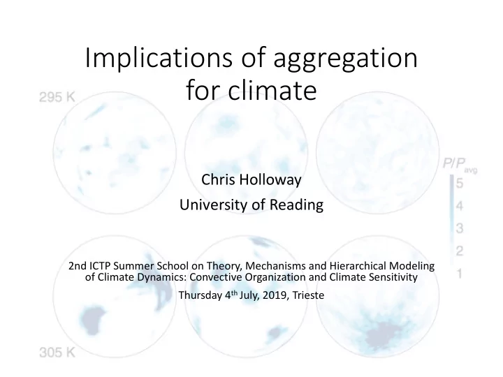
SST dependence of aggregation Khairoutdinov and Emanuel 2010: aggregation only occurs above an SST threshold of 298 K: Proposed a hypothesis of self-organized criticality where: higher SSTs -> agg. -> larger OLR -> lower SSTs -> disagg. -> lower OLR -> higher SSTs and so on. So aggregation would act to maintain tropical SSTs in main convective regions around a critical value around 300 K, similar to observed current climate.
SST dependence of aggregation Emanuel et al. 2014 present a possible mechanism to explain this SST threshold for self-aggregation: Low SST: drying High SST: causes drying clear-sky LW causes warming clear-sky LW cooling And low-level cooling in dry subsidence regions is a critical mechanism for early stages of self-aggregation (Muller and Held 2012, Muller and Bony 2015)
But some complications … Several studies later show that self-aggregation can Abbot 2014 (~ 250 K ) occur at SSTs that are much lower than 298 K: Wing and Cronin 2016 ( 280 K ) Coppin and Bony 2015 ( 292 K ) Holloway and Woolnough 2016 ( 290 K )
But some complications … Although observational studies agree that OLR increases with • increased organisation/aggregation, they are not conclusive on the change in total surface forcing (including SW radiation and turbulent fluxes) that is associated with increased aggregation (Tobin et al. 2012, 2013) The Emanuel et al. (2014) mechanism is valid for clear sky radiation, • but low clouds play an important role in radiative cooling in dry subsidence regions that helps early stages of self-aggregation (including in low-SST simulations): (Muller and Held 2012, Wing and Cronin 2016, Holloway and Woolnough 2016) There is some evidence of self-aggregation not occurring above a • high enough SST threshold, although this may be due to domain-size limitations (Wing and Emanuel 2014)
Ocean coupling Most studies of self-aggregation use atmosphere-only simulations with prescribed SST. However, ocean coupling is highly relevant for climate implications. Hohenegger and Stevens (2016) show that shallow slab oceans lead to reduced self-aggregation due to cloud shading, which cools the surface beneath convective clusters: Hohenegger and Stevens (2016) also found that aggregation stabilised climate and that convection permitting simulations had very different climate sensitivity compared to parameterised convection simulations.
Different mechanisms for different SSTs? (Review) Low SST High SST Coppin and Bony (2015)
Dependence on convection representation and entrainment? Review: Becker et al. (2017) find that convective parameterisation (on/off, and entrainment mixing value) affect SST dependence of aggregation in a global model: They also find that WISHE (wind-evaporation feedback) is important at low SSTs but not at high SSTs (for parameterised convection), where evaporation is higher in dry regions. On the other hand, moisture-convection feedbacks become more important at higher SSTs because larger saturation deficits lead to more dry air dilution per mixing amount.
Anvil cloud effects Bony et al. (2016): • Anvil cloud tops reach higher altitude with warming (the positive cloud altitude effect), but also shrink in size
Anvil cloud effects Bony et al. (2016): • The shrinking is related to increased upper-level stability due to a warmer moist adiabat, which means less clear- sky subsidence per radiative cooling amount and less upper-level divergence meaning less anvil spread (a stability-iris effect ) Relationship between the anvil cloud fraction and the radiatively driven divergence D r predicted by three GCMs in simulations forced by a range of SSTs (colours ranging from blue to red correspond to increasing SST, and each GCM is associated with a different marker). The dashed line represents the linear regression line across all points.
Recommend
More recommend