IMAGE WARPING Vuong Le Dept. Of ECE University of Illinois ECE - PowerPoint PPT Presentation

IMAGE WARPING Vuong Le Dept. Of ECE University of Illinois ECE 417 – Spring 2013 With some slides from Alexei Efros, Steve Seitz, Jilin Tu, and Hao Tang

Content • Introduction • Parametric warping • Barycentric coordinates • Interpolation • MP 6

Content • Introduction • Parametric warping • Barycentric coordinates • Interpolation • MP 6

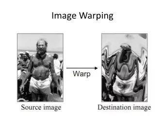
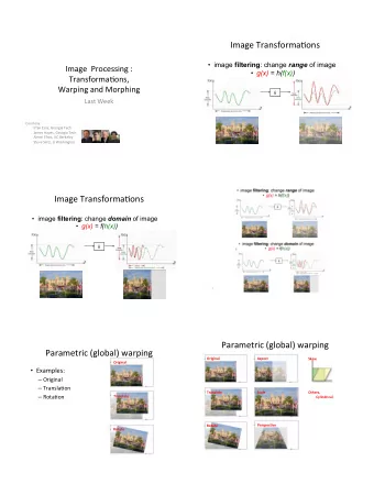
Image Warping image filtering: change range of image g(x) = T(f(x)) f g T x x image warping: change domain of image g(x) = f(T(x)) f g T x x

Image Warping image filtering: change range of image g(x) = T(f(x)) f g T image warping: change domain of image g(x) = f(T(x)) f g T

Global parametric image warping Examples of parametric warps: aspect rotation translation perspective cylindrical affine

Piecewise parametric image warping • Define a mesh of small shape units: triangles/quadrangles • Apply different transformations for different units M1 M2

Non-parametric warping • Move control points of a grid • Use thin plate splines to produces a smooth vector field

Image morphing

Photoshop examples

Photoshop examples

Content • Introduction • Parametric warping • Barycentric coordinates • Interpolation • MP 6

Parametric image warping T p = (x,y) p’ = (x’,y’) Transformation T is a coordinate-changing machine: What does it mean that T is parametric? ° can be described by just a few numbers (parameters) How to represent global and local transforms? ° Global: T Is the same for any point p in the image ° Local: T can be different at different location Let’s try to represent T as a matrix: p’ = M p     x ' x =   M       y ' y

Scaling = Scaling operation: x ' ax = y ' by Or, in matrix form:       x ' a 0 x =             y ' 0 b y scaling matrix S

2-D Rotation (x’, y’) x’ = x cos ( θ ) - y sin ( θ ) (x, y) y’ = x sin ( θ ) + y cos ( θ ) ( ) ( ) θ − θ       x ' cos sin x =       ( ) ( ) θ θ θ       y ' sin cos y R

Shearing in x  The y coordinates are unaffected, but the x coordinates are translated linearly with y  That is = +       x ' 1 sh x x ' x sh * y = y y       =       y ' y y ' 0 1 y

Shearing in y   =     1 0 x ' x x ' x =       = + y ' sh * x y       y ' sh 1 y x x

2x2 Matrices What types of transformations can be represented with a 2x2 matrix? 2D Shear?       = + sh 1 x x x ' x sh * y ' = x x       = + y sh x y ' *   sh   1 y '   y y y 2D Mirror about Y axis? −      x ' 1 0 x = − = x ' x       =       y ' 0 1 y y ' y 2D Mirror over (0,0)? −       x ' 1 0 x = − = x ' x −             = − y ' 0 1 y y ' y

2x2 Matrices What types of transformations can be represented with a 2x2 matrix? 2D Translation? = + x x t ' x NO! = + y ' y t y Only linear 2D transformations can be represented with a 2x2 matrix

All 2D Linear Transformations Linear transformations are combinations of … ° Scale,       x ' a b x ° Rotation, =       ° Shear, and       y ' c d y ° Mirror Properties of linear transformations: ° Origin maps to origin ° Lines map to lines ° Parallel lines remain parallel ° Distance or length ratios are preserved on parallel lines ° Ratios of areas are preserved

Homogeneous Coordinates Q: How can we represent translation as a 3x3 matrix? = + x ' x t x = + y ' y t y

Homogeneous Coordinates Q: How can we represent translation as a 3x3 matrix? = + x x t ' x = + y ' y t y   t 1 0 x   A: Using the rightmost column: = T ranslation 0 1 t   y   0 0 1         x ' 1 0 t x x       =  y ' 0 1 t * y      y           1 0 0 1 1  

Homogeneous Coordinates Add a 3rd coordinate to every 2D point ° (x, y, w) represents a point at location (x/w, y/w) ° (x, y, 0) represents a point at infinity ° (0, 0, 0) is not allowed • Convenient coordinate system to represent many useful transformations • (aw, bw, w) represent the same 2D point for any value of w y 2 1 (2,1,1) or (4,2,2) or (6,3,3) x 2 1

Basic 2D Transformations Basic 2D transformations as 3x3 matrices             x ' s 0 0 x x ' 1 0 t x x x             = = y ' 0 s 0 y y ' 0 1 t y             y y                         1 0 0 1 1 1 0 0 1 1 Translate Scale Θ − Θ             x ' cos sin 0 x x ' 1 sh 0 x x             = Θ Θ = y ' sin cos 0 y y ' sh 1 0 y             y                  1  0 0 1 1       1 0 0 1 1 Rotate Shear

Affine Transformations Affine transformations are combinations of …       x a a a u ° Linear 2D transformations, and 1 2 0       = ° Translations y b b b v       1 2 0 Properties of affine transformations:             1 0 0 1 1 ° Origin does not necessarily map to origin ° Lines map to lines ° Parallel lines remain parallel ° Length/distance ratios are preserved on parallel lines ° Ratios of areas are preserved

Solution to Affine Warping       x a a a u 1 2 0       = y b b b v       1 2 0             1 0 0 1 1

“Triangle-wise” parametric image warping • For each transformed image frame ° Define a mesh of triangles ° Find a affine transform from each triangle’s vertices, apply it to other points inside the triangle  Have to solve affine transforms at every frame M1 M2

Content • Introduction • Parametric warping • Barycentric coordinates • Interpolation • MP 6

Affine warping for triangles

Barycentric Coordinates

Barycentric Coordinates Fact

Content • Introduction • Parametric warping • Barycentric coordinates • Interpolation • MP 6

Image Warping Implementation I

Forward Mapping

Forward Mapping

Forward Mapping

Image Warping Implementation II

Reverse Mapping

Resampling Evaluate source image at arbitrary (u, v) ° (u, v) does not usually have integer coordinates Some kinds of resampling ° Nearest neighbor ° Bilinear interpolation ° Gaussian filter Source Image Destination Image

Nearest neighbor Take value at closest pixel int iu = trunc(u + 0.5); int iv = trunc(v + 0.5); dst(x, y) = src(iu, iv); Simple, but causes aliasing

Bilinear interpolation Bilinearly interpolate four surrounding pixels a = linear interpolation of src(u 1 , v 1 ) and src(u 2 , v 1 ) b = linear interpolation of src(u 1 , v 2 ) and src(u 2 , v 2 ) dst(x, y) = linear interpolation of ‘a’ and ‘b’ a (u1,v1) (u2,v1) (x,y) (u2,v2) (u1,v2) b

Gaussian Filter Convolve with Gaussian filter Width of Gaussian kernel affects bluriness

Image Warping Implementation II – with resampling

Image Warping Implementation II – with Gaussian resampling

Content • Introduction • Parametric warping • Barycentric coordinates • Interpolation • MP 6

Warping in MP 6 • Warping ° For each triangle find the affine transform ° Apply it to the points inside ° Assign image value to the triangle points • Suggestions ° Barycentric coordinate ° Reverse mapping

Preview of MP 6