Image warping/morphing Digital Visual Effects, Spring 2006 Yung-Yu - PowerPoint PPT Presentation

Image warping/morphing Digital Visual Effects, Spring 2006 Yung-Yu Chuang 2005/3/15 with slides by Richard Szeliski, Steve Seitz and Alexei Efros

Outline • Images • Image warping • Image morphing

Image fundamentals

B A Image formation

Sampling and quantization

What is an image 2 � R: • We can think of an image as a function, f : R – f ( x, y ) gives the intensity at position ( x, y ) – defined over a rectangle, with a finite range: • f : [ a , b ]x[ c , d ] � [0,1] f x y ⎡ ⎤ r ( x , y ) • A color image ⎢ ⎥ = ⎢ ( , ) ( , ) f x y g x y ⎥ ⎢ ⎥ ⎣ ⎦ b x ( , y )

A digital image • We usually operate on digital ( discrete ) images: – Sample the 2D space on a regular grid – Quantize each sample (round to nearest integer) • If our samples are D apart, we can write this as: f [ i , j ] = Quantize{ f ( i D, j D) } • The image can now be represented as a matrix of integer values 62 79 23 119 120 105 4 0 10 10 9 62 12 78 34 0 10 58 197 46 46 0 0 48 176 135 5 188 191 68 0 49 2 1 1 29 26 37 0 77 0 89 144 147 187 102 62 208 255 252 0 166 123 62 0 31 166 63 127 17 1 0 99 30

Image warping

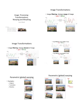
Image warping image filtering: change range of image g(x) = h(f(x)) f g h x x image warping: change domain of image g(x) = f(h(x)) f g h x x

Image warping image filtering: change range of image f(x) = h(g(x)) f g h image warping: change domain of image f(x) = g(h(x)) f g h

Parametric (global) warping Examples of parametric warps: aspect rotation translation perspective cylindrical affine

Parametric (global) warping T p = (x,y) p’ = (x’,y’) • Transformation T is a coordinate-changing machine: p ’ = T (p) • What does it mean that T is global? – Is the same for any point p – can be described by j ust a few numbers (parameters) • Represent T as a matrix: p ’ = M *p ⎡ ⎤ ⎡ ⎤ ' x x = ⎢ ⎥ M ⎢ ⎥ ⎣ ⎦ ⎣ ⎦ ' y y

Scaling • S caling a coordinate means multiplying each of its components by a scalar • Uniform scaling means this scalar is the same for all components: × 2

Scaling • Non-uniform scaling : different scalars per component: X × 2, Y × 0.5

Scaling = x ' ax • S caling operation: = y ' by • Or, in matrix form: ⎡ ⎤ ⎡ ⎤ ⎡ ⎤ ' 0 x a x = ⎢ ⎥ ⎢ ⎥ ⎢ ⎥ ⎣ ⎦ ⎣ ⎦ ⎣ ⎦ ' 0 y b y scaling matrix S What’s inverse of S?

2-D Rotation • This is easy to capture in matrix form: ( ) ( ) θ − θ ⎡ ⎤ ⎡ ⎤ ⎡ ⎤ ' cos sin x x = ⎢ ⎥ ⎢ ⎥ ⎢ ⎥ ( ) ( ) θ θ ⎣ ⎦ ⎣ ⎦ ⎣ ⎦ ' sin cos y y R Even though sin( θ ) and cos( θ ) are nonlinear to θ , • – x ’ is a linear combination of x and y – y ’ is a linear combination of x and y • What is the inverse transformation? – Rotation by – θ − 1 = T – For rotation matrices, det(R) = 1 so R R

2x2 Matrices • What types of transformations can be represented with a 2x2 matrix? 2D Identity? = ⎡ ⎤ ⎡ ⎤ ⎡ ⎤ x ' 1 0 x ' x x = ⎢ ⎥ ⎢ ⎥ ⎢ ⎥ = ⎣ ⎦ ⎣ ⎦ ⎣ ⎦ y ' 0 1 y y ' y 2D Scale around (0,0)? = ⎡ ⎤ x ' s * x ⎡ ⎤ ⎡ ⎤ s 0 x ' x x = x ⎢ ⎥ ⎢ ⎥ ⎢ ⎥ = y ' s * y ⎣ ⎦ s ⎣ ⎦ 0 y ' ⎣ ⎦ y y y

2x2 Matrices • What types of transformations can be represented with a 2x2 matrix? 2D Rotate around (0,0)? = θ − θ θ − θ ⎡ ⎤ ⎡ ⎤ ⎡ ⎤ x ' cos * x sin * y x ' cos sin x = ⎢ ⎥ ⎢ ⎥ ⎢ ⎥ = θ + θ θ θ y ' sin * x cos * y ⎣ ⎦ ⎣ ⎦ ⎣ ⎦ y ' sin cos y 2D Shear? ⎡ ⎤ = + ⎡ ⎤ ⎡ ⎤ 1 sh x ' x sh * y x x ' = x x ⎢ ⎥ ⎢ ⎥ ⎢ ⎥ = + y ' sh * x y sh ⎣ ⎦ 1 ⎣ ⎦ y ' ⎣ ⎦ y y y

2x2 Matrices • What types of transformations can be represented with a 2x2 matrix? 2D Mirror about Y axis? ⎡− ⎡ ⎤ ⎤ ⎡ ⎤ = − x ' 1 0 x = x ' x ⎢ ⎥ ⎢ ⎥ ⎢ ⎥ = ⎣ ⎦ ⎣ ⎦ ⎣ ⎦ ' 0 1 y y ' y y 2D Mirror over (0,0)? − ⎡ ⎤ ⎡ ⎤ ⎡ ⎤ = − x ' 1 0 x x ' x = − = − ⎢ ⎥ ⎢ ⎥ ⎢ ⎥ ⎣ ⎦ ⎣ ⎦ ⎣ ⎦ ' y ' 0 1 y y y

All 2D Linear Transformations • Linear transformations are combinations of … – S cale, – Rotation, – S hear, and – Mirror • Properties of linear transformations: – Origin maps to origin – Lines map to lines – Parallel lines remain parallel – Ratios are preserved ⎡ ⎤ ⎡ ⎤ ⎡ ⎤ x ' a b x – Closed under composition = ⎢ ⎥ ⎢ ⎥ ⎢ ⎥ ⎣ ⎦ ⎣ ⎦ ⎣ ⎦ y ' c d y

2x2 Matrices • What types of transformations can be represented with a 2x2 matrix? 2D Translation? = + x ' x t x NO! = + y ' y t y Only linear 2D transformations can be represented with a 2x2 matrix

Translation • Example of translation Homogeneous Coordinates ⎡ ⎤ + ⎡ ⎤ ⎡ ⎤ ⎡ ⎤ x ' 1 0 t x x t x x ⎢ ⎥ ⎢ ⎥ ⎢ ⎥ ⎢ ⎥ = = + y ' 0 1 t y y t ⎢ ⎥ ⎢ ⎥ ⎢ ⎥ ⎢ ⎥ y y ⎢ ⎥ ⎢ ⎥ ⎢ ⎥ ⎢ ⎥ ⎣ ⎦ ⎣ ⎦ ⎣ ⎦ 1 0 0 1 1 1 ⎣ ⎦ t x = 2 t y = 1

Affine Transformations • Affine transformations are combinations of … – Linear transformations, and – Translations • Properties of affine transformations: – Origin does not necessarily map to origin – Lines map to lines – Parallel lines remain parallel – Ratios are preserved ⎡ ⎤ ⎡ ⎤ ⎡ ⎤ – Closed under composition x ' a b c x – Models change of basis ⎢ ⎥ ⎢ ⎥ ⎢ ⎥ = y ' d e f y ⎢ ⎥ ⎢ ⎥ ⎢ ⎥ ⎣ ⎦ ⎣ ⎦ ⎣ ⎦ w 0 0 1 w

Projective Transformations • Proj ective transformations … – Affine transformations, and – Proj ective warps • Properties of proj ective transformations: – Origin does not necessarily map to origin – Lines map to lines – Parallel lines do not necessarily remain parallel – Ratios are not preserved – Closed under composition ⎡ ⎤ ⎡ ⎤ ⎡ ⎤ ' x a b c x – Models change of basis ⎢ ⎥ ⎢ ⎥ ⎢ ⎥ = y ' d e f y ⎢ ⎥ ⎢ ⎥ ⎢ ⎥ ⎣ ⎦ ⎣ ⎦ ⎣ ⎦ ' w g h i w

2D coordinate transformations x = ( x , y ) • translation: x’ = x + t x’ = R x + t • rotation: x’ = s R x + t • similarity: • affine: x’ = A x + t x’ ≅ H x x = ( x , y ,1) • perspective: ( x is a homogeneous coordinate) • These all form a nested group (closed under composition w/ inv.)

Image warping • Given a coordinate transform x ’ = h ( x ) and a source image f ( x ), how do we compute a transformed image g ( x ’ ) = f ( h ( x ))? h ( x ) x x’ f ( x ) g ( x’ )

Forward warping • S end each pixel f ( x ) to its corresponding location x’ = h ( x ) in g ( x’ ) h ( x ) x x’ f ( x ) g ( x’ )

Forward warping • S end each pixel f ( x ) to its corresponding location x’ = h ( x ) in g ( x’ ) • What if pixel lands “between” two pixels? • Answer: add “contribution” to several pixels, normalize later ( splatting ) h ( x ) x x’ f ( x ) g ( x’ )

Inverse warping • Get each pixel g ( x’ ) from its corresponding location x = h -1 ( x’ ) in f ( x ) h -1 ( x’ ) x x’ f ( x ) g ( x’ )

Inverse warping • Get each pixel g ( x’ ) from its corresponding location x = h -1 ( x’ ) in f ( x ) • What if pixel comes from “between” two pixels? • Answer: resample color value from interpolated ( prefiltered ) source image x x’ f ( x ) g ( x’ )

Interpolation • Possible interpolation filters: – nearest neighbor – bilinear – bicubic – sinc / FIR

• A simple method for resampling images Bilinear interpolation

Non-parametric image warping • S pecify a more detailed warp function • S plines, meshes, optical flow (per-pixel motion)

Demo • http:/ / www.colonize.com/ warp/ • Warping is a useful operation for mosaics, video matching, view interpolation and so on.

Image morphing

Image morphing • The goal is to synthesize a fluid transformation from one image to another. • Cross dissolving is a common transition between cuts, but it is not good for morphing because of the ghosting effects. image #2 image #1 dissolving

http:/ / www.salavon.com/ Artifacts of cross-dissolving

Image morphing • Why ghosting? • Morphing = warping + cross-dissolving shape color (geometric) (photometric)

Image morphing image #1 cross-dissolving image #2 warp warp morphing

Morphing sequence

average faces Face averaging by morphing

Image morphing create a morphing sequence: for each time t 1. Create an intermediate warping field (by interpolation) 2. Warp both images towards it 3. Cross-dissolve the colors in the newly warped images

t=1 morphing t=0.75 t=0.25 t=0.5 An ideal example t=0

t=1 middle face (t=0.5) An ideal example t=0