Image warping and stitching Tues Mar 20 Kristen Grauman UT Austin - PDF document
CS 376 Computer Vision: lecture 15 3/19/2018 Image warping and stitching Tues Mar 20 Kristen Grauman UT Austin Last time Feature-based alignment 2D transformations Affine fit RANSAC Robust feature-based alignment Source:
CS 376 Computer Vision: lecture 15 3/19/2018 Image warping and stitching Tues Mar 20 Kristen Grauman UT Austin Last time • Feature-based alignment – 2D transformations – Affine fit – RANSAC Robust feature-based alignment Source: L. Lazebnik 1
CS 376 Computer Vision: lecture 15 3/19/2018 Robust feature-based alignment • Extract features Source: L. Lazebnik Robust feature-based alignment • Extract features • Compute putative matches Source: L. Lazebnik Robust feature-based alignment • Extract features • Compute putative matches • Loop: • Hypothesize transformation T (small group of putative matches that are related by T ) Source: L. Lazebnik 2
CS 376 Computer Vision: lecture 15 3/19/2018 Robust feature-based alignment • Extract features • Compute putative matches • Loop: • Hypothesize transformation T (small group of putative matches that are related by T ) • Verify transformation (search for other matches consistent with T ) Source: L. Lazebnik Robust feature-based alignment • Extract features • Compute putative matches • Loop: • Hypothesize transformation T (small group of putative matches that are related by T ) • Verify transformation (search for other matches consistent with T ) Source: L. Lazebnik RANSAC for line fitting example 1. Randomly select minimal subset of points 2. Hypothesize a model 3. Compute error function 4. Select points consistent with model 5. Repeat hypothesize-and- verify loop Source: R. Raguram Lana Lazebnik 3
CS 376 Computer Vision: lecture 15 3/19/2018 How many trials for RANSAC? To ensure good chance of finding true inliers, need sufficient number of trials, S. Let p be probability that any given match is valid Let P be to the total prob of success after S trials. Likelihood in one trial that all k random samples are inliers is p k k p S Likelihood that all S trials will fail is 3 0.5 35 1-P = (1-p k ) S 6 0.6 97 Required minimum number of trials is S = log(1-P) / log(1-p k ) 6 0.5 293 Kristen Grauman Last time: RANSAC for fitting a model (line)… What about fitting a transformation (e.g., translation)? RANSAC: General form • RANSAC loop: 1. Randomly select a seed group on which to base transformation estimate (e.g., a group of matches) 2. Compute transformation from seed group 3. Find inliers to this transformation 4. If the number of inliers is sufficiently large, re-compute estimate of transformation on all of the inliers • Keep the transformation with the largest number of inliers 4
CS 376 Computer Vision: lecture 15 3/19/2018 RANSAC example: Translation Putative matches Source: Rick Szeliski RANSAC example: Translation Select one match, count inliers RANSAC example: Translation Select one match, count inliers 5
CS 376 Computer Vision: lecture 15 3/19/2018 RANSAC example: Translation Find “average” translation vector Another example Automatic scanned document rotater using Hough lines and RANSAC https://www.youtube.com/watch?v=O0v9FAk43 kY RANSAC pros and cons • Pros • Simple and general • Applicable to many different problems • Often works well in practice • Cons • Parameters to tune • Doesn’t work well for low inlier ratios (too many iterations, or can fail completely) • Can’t always get a good initialization of the model based on the minimum number of samples Slide credit: Lana Lazebnik 6
CS 376 Computer Vision: lecture 15 3/19/2018 Today • Image mosaics – Fitting a 2D transformation • Affine, Homography – 2D image warping – Computing an image mosaic Mosaics . . . image from S. Seitz Obtain a wider angle view by combining multiple images. Main questions Alignment : Given two T images, what is the transformation between them? Warping : Given a T source image and a transformation, what does the transformed output look like? 7
CS 376 Computer Vision: lecture 15 3/19/2018 2D Affine Transformations x ' a b c x y ' d e f y w ' 0 0 1 w Affine transformations are combinations of … • Linear transformations, and • Translations Parallel lines remain parallel Projective Transformations x ' a b c x y ' d e f y w ' g h i w Projective transformations: • Affine transformations, and • Projective warps Parallel lines do not necessarily remain parallel 2D transformation models • Similarity (translation, scale, rotation) • Affine • Projective (homography) 8
CS 376 Computer Vision: lecture 15 3/19/2018 How to stitch together a panorama (a.k.a. mosaic)? • Basic Procedure – Take a sequence of images from the same position • Rotate the camera about its optical center – Compute transformation between second image and first – Transform the second image to overlap with the first – Blend the two together to create a mosaic – (If there are more images, repeat) • …but wait , why should this work at all? – What about the 3D geometry of the scene? – Why aren’t we using it? Source: Steve Seitz Pinhole camera • Pinhole camera is a simple model to approximate imaging process, perspective projection . Image plane Virtual pinhole image If we treat pinhole as a point, only one ray from any given point can enter the camera. Fig from Forsyth and Ponce Mosaics . . . image from S. Seitz Obtain a wider angle view by combining multiple images. 9
CS 376 Computer Vision: lecture 15 3/19/2018 Mosaics: generating synthetic views real synthetic camera camera Can generate any synthetic camera view as long as it has the same center of projection ! Source: Alyosha Efros Image reprojection mosaic PP The mosaic has a natural interpretation in 3D • The images are reprojected onto a common plane • The mosaic is formed on this plane • Mosaic is a synthetic wide-angle camera Source: Steve Seitz Image reprojection Basic question • How to relate two images from the same camera center? – how to map a pixel from PP1 to PP2 PP2 Answer • Cast a ray through each pixel in PP1 • Draw the pixel where that ray intersects PP2 PP1 Observation: Rather than thinking of this as a 3D reprojection, think of it as a 2D image warp from one image to another. Source: Alyosha Efros 10
CS 376 Computer Vision: lecture 15 3/19/2018 Image reprojection: Homography A projective transform is a mapping between any two PPs with the same center of projection • rectangle should map to arbitrary quadrilateral • parallel lines aren’t • but must preserve straight lines called Homography PP2 wx' * * * x PP1 wy' * * * y * * * w 1 p’ H p Source: Alyosha Efros Homography x 1 , y x 1 , y 1 1 x 2 , y x 2 , y 2 2 … … , x , n y x n y n n To compute the homography given pairs of corresponding points in the images, we need to set up an equation where the parameters of H are the unknowns… Solving for homographies p’ = Hp wx' a b c x wy' d e f y w g h i 1 Can set scale factor i =1. So, there are 8 unknowns. Set up a system of linear equations: Ah = b where vector of unknowns h = [a,b,c,d,e,f,g,h] T Need at least 8 eqs, but the more the better… Solve for h. If overconstrained, solve using least-squares: 2 Ah min b >> help lmdivide BOARD 11
CS 376 Computer Vision: lecture 15 3/19/2018 Homography w y x , y w x w , w x , y wx' * * * x To apply a given homography H wy' * * * y • Compute p’ = Hp (regular matrix multiply) • Convert p’ from homogeneous to image * * * w 1 coordinates p p’ H RANSAC for estimating homography RANSAC loop: 1. Select four feature pairs (at random) 2. Compute homography H 3. Compute inliers where SSD(p i ’, H p i )< ε 4. Keep largest set of inliers 5. Re-compute least-squares H estimate on all of the inliers Slide credit: Steve Seitz Today • Image mosaics – Fitting a 2D transformation • Affine, Homography – 2D image warping – Computing an image mosaic 12
CS 376 Computer Vision: lecture 15 3/19/2018 A2 Examples Scott Staniewicz Color + Texture EC Andrew Romanyk Radius 38, Bin Size 1 Variable Radius EC 90% threshold 13
CS 376 Computer Vision: lecture 15 3/19/2018 Po-Chen Wu Po-Chen Wu Christopher Gamberg 5 Regions, 25 Window Size 14
CS 376 Computer Vision: lecture 15 3/19/2018 Christopher Gamberg All Filters Only Blob Filters Thomas Lam William Kuglen 15
CS 376 Computer Vision: lecture 15 3/19/2018 William Kuglen Kurtis David Veronica Gunn 16
CS 376 Computer Vision: lecture 15 3/19/2018 Michael Li Benjamin Yang Brahma Pavse 17
Recommend
More recommend
Explore More Topics
Stay informed with curated content and fresh updates.
