Image Smoothing ! Chicken-and-egg dilemma! " ! Edge preserving - PowerPoint PPT Presentation

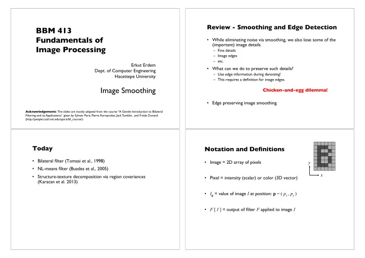
Review - Smoothing and Edge Detection " BBM 413 ! Fundamentals of ! • While eliminating noise via smoothing, we also lose some of the (important) image details. ! Image Processing ! – Fine details ! – Image edges ! – etc. ! Erkut Erdem " • What can we do to preserve such details? ! Dept. of Computer Engineering " – Use edge information during denoising! ! Hacettepe University " – This requires a definition for image edges. ! ! ! Image Smoothing ! Chicken-and-egg dilemma! " ! • Edge preserving image smoothing ! Acknowledgement: The slides are mostly adapted from the course “A Gentle Introduction to Bilateral " Filtering and its Applications” given by Sylvain Paris, Pierre Kornprobst, Jack Tumblin, and Frédo Durand " (http://people.csail.mit.edu/sparis/bf_course/) ! Today " Notation and Definitions " • Bilateral filter (Tomasi et al., 1998) ! • Image = 2D array of pixels ! y • NL-means filter (Buades et al., 2005) ! x • Structure-texture decomposition via region covariances • Pixel = intensity (scalar) or color (3D vector) ! (Karacan et al. 2013) ! • I p = value of image I at position: p = ( p x , p y ) • F [ I ] = output of filter F applied to image I

Strategy for Smoothing Images " Box Average " • Images are not smooth because " adjacent pixels are different. ! square neighborhood ! • Smoothing = making adjacent pixels " ! ! ! look more similar. ! output ! input ! • Smoothing strategy " ! pixel as average of its neighbors ! average ! Square Box Generates Defects " Equation of Box Average " • Axis-aligned streaks ! ∑ = − • Blocky results ! BA [ I ] B ( p q ) I output ! σ p q ∈ q S intensity at " result at " pixel q " pixel p " sum over " input ! all pixels q " normalized " box function ! 0 !

Strategy to Solve these Problems " Gaussian Blur " per-pixel multiplication ! • Use an isotropic ( i.e. circular) window. ! • Use a window with a smooth falloff. ! * ! input ! output ! average ! box window ! Gaussian window ! input " box average "

Gaussian blur " Equation of Gaussian Blur " Same idea: weighted average of pixels . ! ( ) ∑ = − GB [ I ] G || p q || I σ p q ∈ q S normalized " Gaussian function ! 1 ! 0 ! How to set s ! Spatial Parameter " • Depends on the application. ! ( ) ∑ = − GB [ I ] G || p q || I input ! σ p q ∈ q S • Common strategy: proportional to image size ! size of the window ! – e.g. 2% of the image diagonal ! – property: independent of image resolution ! small s ! large s ! limited smoothing ! strong smoothing !

Properties of Gaussian Blur " Properties of Gaussian Blur " input ! • Weights independent of spatial location ! • Does smooth images ! • But smoothes too much: " – linear convolution ! edges are blurred . ! – Only spatial distance matters ! – well-known operation ! – No edge term ! – efficient computation (recursive algorithm, FFT…) ! output ! ∑ ( ) = − GB [ I ] G || p q || I σ p q ∈ q S space ! [Aurich 95, Smith 97, Tomasi 98] ! Blur Comes from ! Bilateral Filter ! Averaging across Edges " No Averaging across Edges " * ! * ! input ! output ! input ! output ! * ! * ! * ! * ! Same Gaussian kernel everywhere. ! The kernel shape depends on the image content. !

Illustration a 1D Image " Bilateral Filter Definition: ! an Additional Edge Term " • 1D image = line of pixels ! Same idea: weighted average of pixels . ! new ! not new ! new ! ( ) 1 ( ) ∑ = − − BF [ I ] G || p q || G | I I | I σ σ p p q q • Better visualized as a plot ! W s r ∈ q S p normalization " space weight ! range weight ! pixel ! factor ! intensity " I ! pixel position " Gaussian Blur and Bilateral Filter " Bilateral Filter on a Height Field " Gaussian blur ! ( ) 1 ( ) ∑ = − − BF [ I ] G || p q || G | I I | I σ σ p p q q W s r p " ∈ p q S ( ) ∑ = − GB [ I ] G || p q || I q " σ p q q ∈ S space ! space ! p p Bilateral filter " q [Aurich 95, Smith 97, Tomasi 98] ! p " 1 ( ) range ! ( ) ∑ = − − BF [ I ] G || p q || G | I I | I p σ σ p q q W q " s r ∈ q S p space ! range ! output ! input ! normalization ! space ! reproduced ! from [Durand 02] "

Influence of Pixels " Space and Range Parameters " Only pixels close in space and in range are considered. ! ( ) 1 ( ) ∑ = − − BF [ I ] G || p q || G | I I | I space ! σ σ p p q q W s r ∈ q S p • space s s : spatial extent of the kernel, size of the considered range ! neighborhood. ! p " • range s r : “ minimum ” amplitude of an edge ! Exploring the Parameter Space " Varying the Range Parameter " s r = � " s r = � " s r = 0.1 ! s r = 0.25 ! s r = 0.1 ! s r = 0.25 ! (Gaussian blur) ! (Gaussian blur) ! input ! input ! s s = 2 ! s s = 2 ! s s = 6 ! s s = 6 ! s s = 18 ! s s = 18 !

s r = 0.1 " input " s r = 0.25 " s r = � ! (Gaussian blur) "

Varying the Space Parameter " input " s r = � " s r = 0.1 ! s r = 0.25 ! (Gaussian blur) ! input ! s s = 2 ! s s = 6 ! s s = 18 ! s s = 2 " s s = 6 "

s s = 18 " How to Set the Parameters " Depends on the application. For instance: ! ! • space parameter: proportional to image size ! – e.g., 2% of image diagonal ! • range parameter: proportional to edge amplitude ! – e.g., mean or median of image gradients ! • independent of resolution and exposure ! Bilateral Filter Crosses Thin Lines " Iterating the Bilateral Filter " • Bilateral filter averages across " ! features thinner than ~2 s s ! = • Desirable for smoothing: more pixels = more robust ! I BF [ I ] + ( n 1 ) ( n ) • Different from diffusion that stops at thin lines ! • Generate more piecewise-flat images ! close-up ! kernel ! • Often not needed in computational photo. !

input " 1 iteration " 2 iterations " 4 iterations "

Hard to Compute " Bilateral Filtering Color Images " ( ) • Nonlinear ! 1 ∑ ( ) = − − BF [ I ] G || p q || G | I I | I input ! σ σ p p q q W s r For gray-level images ! intensity difference ! ∈ p q S ( ) 1 ( ) ∑ = − − • Complex, spatially varying kernels ! BF [ I ] G || p q || G | I I | I σ σ p p q q W s r q ∈ S – Cannot be precomputed, no FFT… ! p scalar ! output ! For color images ! color difference ! ( ) 1 ∑ ( ) = − − BF [ I ] G || p q || G || C C || C σ σ p p q q W s r ∈ q S p 3D vector " (RGB, Lab) ! • Brute-force implementation is slow > 10min ! Basic denoising " Basic denoising " Noisy input ! Bilateral filter 7x7 window ! Bilateral filter ! Median 3x3 !

Basic denoising " Basic denoising " Bilateral filter ! Median 5x5 ! Bilateral filter ! Bilateral filter – lower sigma ! Basic denoising " Denoising " Bilateral filter ! Bilateral filter – higher sigma ! • Small spatial sigma (e.g. 7x7 window) ! • Adapt range sigma to noise level ! • Maybe not best denoising method, but best simplicity/quality tradeoff ! – No need for acceleration (small kernel) ! – But the denoising feature in e.g. Photoshop is better !

New Idea: ! Goal: Understand how does bilateral filter relates with other methods ! NL-Means Filter (Buades 2005) " Bilateral ! • Same goals: ‘ Smooth within Similar Regions ’ ! filter ! • KEY INSIGHT : Generalize, extend ‘ Similarity ’ ! Partial ! – Bilateral: " Local mode ! ! Averages neighbors with similar intensities ; ! differential ! filtering ! equations ! – NL-Means: " Averages neighbors with similar neighborhoods! " Robust ! statistics ! more in BIL717 Image Processing graduate course.. ! NL-Means Method: ! NL-Means Method: ! Buades (2005) " Buades (2005) " ! ! ! • For each and ! • For each and ! every pixel p: " every pixel p: ! " " " – Define a small, simple fixed size neighborhood; !

NL-Means Method: ! NL-Means Method: ! Buades (2005) " Buades (2005) " q ! ‘ Similar ’ pixels p, q " 0.74 ! ! 0.32 ! ! SMALL ! V p = " 0.41 ! vector distance; ! 0.55 ! … ! … ! p ! ! … ! || V p – V q || 2 " • For each and ! ! every pixel p: ! ! " – Define a small, simple fixed size neighborhood; ! – Define vector V p : a list of neighboring pixel values. ! NL-Means Method: ! NL-Means Method: ! Buades (2005) " Buades (2005) " q ! ‘ Dissimilar ’ pixels p, q " ‘ Dissimilar ’ pixels p, q " ! LARGE ! ! LARGE ! vector distance; ! vector distance; ! q ! q ! p ! p ! ! ! || V p – V q || 2 " || V p – V q || 2 " ! ! ! Filter with this! " "