Smoothing In image processing literature, the weighting averaging - PowerPoint PPT Presentation
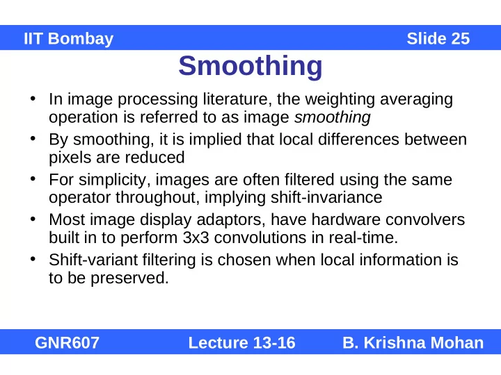
IIT Bombay Slide 25 Smoothing In image processing literature, the weighting averaging operation is referred to as image smoothing By smoothing, it is implied that local
IIT Bombay Slide 25 Smoothing • In image processing literature, the weighting averaging operation is referred to as image smoothing • By smoothing, it is implied that local differences between pixels are reduced • For simplicity, images are often filtered using the same operator throughout, implying shift-invariance • Most image display adaptors, have hardware convolvers built in to perform 3x3 convolutions in real-time. • Shift-variant filtering is chosen when local information is to be preserved. GNR607 Lecture 13-16 B. Krishna Mohan
IIT Bombay Slide 26 Original Image GNR607 Lecture 13-16 B. Krishna Mohan
IIT Bombay Slide 27 3x3 averaging GNR607 Lecture 13-16 B. Krishna Mohan
IIT Bombay Slide 28 Gaussian smoothing • Gaussian filter: linear smoothing • weight matrix 2 2 + 1 r c − ( ) = 2 σ w ( r , c ) ke 2 1 = k ∈ ( r , c ) W , for all where 2 2 + 1 r c − ( ) ∑ 2 e 2 σ ∈ ( r , c ) W W : one or two σ from center GNR607 Lecture 13-16 B. Krishna Mohan
IIT Bombay Slide 28a Gaussian smoothing • Use of Gaussian filter: Specify size of neighborhood size, and given value of σ , determine filter coefficients by varying r,c in the range [–W/2 +W/2] • Alternatively, given value of σ , find the size of the neighbourhood from 3 σ limits • About 99% of the Gaussian distribution is covered within the range mean ± 3 3 σ • r,c vary in the range = [-3 σ + 3 σ ] • For example, if σ = 1, then the range is [-3 3], i.e., the size of neighbourhood is 7x7 GNR607 Lecture 13-16 B. Krishna Mohan
IIT Bombay Slide 28b p(x) Gaussian curve x µ−2σ µ−σ µ µ+σ µ+2σ GNR607 Lecture 13-16 B. Krishna Mohan
IIT Bombay Slide 29 Shift-Variant Filtering • When the filtering operation is required to adapt to the local intensity variations then the filter coefficients should vary according to the position in the image. • Shift-variant filters can preserve the object boundaries better, while smoothing the image • One example is the sigma filter GNR607 Lecture 13-16 B. Krishna Mohan
IIT Bombay Slide 30 Sigma filter • The underlying principle here is to take the subset of pixels in the neighborhood whose gray levels lie within c. σ of the central pixel = + = + k i w l j w = ∑ ∑ g h f − − i j , i j k l , , , i k j l , = − = − k i w l j w • h i,j,k,l = 0 if |f i-j,k=l – f ij | > c. σ ij ; h i,j,k,l = 1 otherwise σ ij is the local standard deviation of the gray levels within the neighborhood centred at pixel (i,j) • To save time, one can also use global std. dev. • c = 1 or 2 depending on the size of neighborhood GNR607 Lecture 13-16 B. Krishna Mohan
IIT Bombay Slide 31 Sigma Filter Algorithm • Consider neighborhood size, and value of c • Find the mean and standard deviation of the pixels within the neighborhood • Find the neighbors of the central pixel whose gray levels are within c. σ of the central pixel’s gray level • Compute the average of the pixels meeting the above criterion • Replace the central pixel’s value by the average • This cannot be replaced by a convolution since the filter response varies for each position in the image GNR607 Lecture 13-16 B. Krishna Mohan
IIT Bombay Slide 31a Comments on Sigma Filter • Degradation of a smoothed image is due to blurring of object boundaries • Here boundaries are better preserved by limiting the smoothing only to a homogeneous subset of pixels in the neighborhood • The selected subset comprises those pixels that have similar intensities • Pixels with very different intensities are excluded by making corresponding weights equal to 0 GNR607 Lecture 13-16 B. Krishna Mohan
IIT Bombay Slide 32 Lee filter Simple Lee filter • g ij = f mean + k.(f ij – f mean ) • k varies between 0 and 2 k = 0, g ij = f mean simple averaging k = 1, g ij = f ij no smoothing at all k = 2, g ij = f ij + (f ij – f mean ) Interpretation of (f ij – f mean ) ??? GNR607 Lecture 13-16 B. Krishna Mohan
IIT Bombay Slide 33 Lee filter a. Original image b. Wallis filter c. K=2 d. K=3 e. K=0.5 f. K=0 GNR607 Lecture 13-16 B. Krishna Mohan
IIT Bombay Slide 34 General form of Lee filter • The general form of Lee filter is given by = + − g f k ( f f ) ij mean ij ij mean • k ij is given by σ 2 ij = k ij σ + σ 2 2 2 f mean v ij • Greater noise, smaller k ij , hence more smoothing GNR607 Lecture 13-16 B. Krishna Mohan
Recommend
More recommend
Explore More Topics
Stay informed with curated content and fresh updates.
