Modelling of turbulent flows: RANS and LES Turbulenzmodelle in der - PowerPoint PPT Presentation
Introduction Filtering More on filtering Modelling of turbulent flows: RANS and LES Turbulenzmodelle in der Str omungsmechanik: RANS und LES Markus Uhlmann Institut f ur Hydromechanik Karlsruher Institut f ur Technologie
Introduction Filtering More on filtering Modelling of turbulent flows: RANS and LES Turbulenzmodelle in der Str¨ omungsmechanik: RANS und LES Markus Uhlmann Institut f¨ ur Hydromechanik Karlsruher Institut f¨ ur Technologie www.ifh.kit.edu SS 2012 Lecture 8 1 / 21
Introduction Filtering More on filtering LECTURE 8 Introduction to Large Eddy Simulation & Spatial Filtering 2 / 21
Introduction Filtering More on filtering Questions to be answered in the present lecture What are the basic elements of the LES approach? How can (explicit) spatial filtering be realized? 3 / 21
Introduction Filtering More on filtering Basic idea of Large-Eddy Simulation ◮ consider the time-dependent Navier-Stokes equations ◮ resolve only the large scales of motion numerically ◮ replace the action of the small scales by a model 4 / 21
Introduction Filtering More on filtering Conceptual steps involved in an LES analysis Intermediate steps 1. define a spatial filter 2. derive the filtered Navier-Stokes equations 3. choose a model for the unclosed subgrid-stress term 4. solve the closed equations numerically Result → approximation of the large-scale motions (single flow realization) 5 / 21
Introduction Generalities Filtering Fourier space More on filtering Discrete data Resolving the large scales in LES physical space spectral space 0 LES DNS 10 −2 10 E ( κ ) −4 10 −6 ∆ x − 1 ∆ x − 1 10 LES DNS −8 DNS LES 10 −2 0 10 10 wavenumber κη 6 / 21
Introduction Generalities Filtering Fourier space More on filtering Discrete data Two different viewpoints of LES & filtering I Explicit filtering (through a filter operation) ◮ spatial filtering, residual stress modelling and numerical solution of the model equations are treated separately II Implicit filtering (by the numerical grid) ◮ numerical discretization errors are deliberately treated as part of the model → we will first consider explicit filtering 7 / 21
Introduction Generalities Filtering Fourier space More on filtering Discrete data Definition of the filter operation General definition � u ( x , t ) = G ( r , x ) u ( x − r , t ) d r (volume integral) � �� � � �� � filter fct. signal � ◮ normalization condition: G ( r , x ) d r = 1 ∀ x + u ′ ( x , t ) ◮ decomposition: u ( x , t ) = u ( x , t ) � �� � � �� � filtered residual → appears analogous to Reynolds decomposition ◮ BUT: u ( x , t ) is a random field! ◮ AND: u ′ � = 0 ALSO: u � = u 8 / 21
Introduction Generalities Filtering Fourier space More on filtering Discrete data Filtering in one spatial dimension ◮ 1D case, consider homogeneous filter functions G ( r ) � ∞ u ( x ) = G ( r ) u ( x − r ) d r −∞ Example from Pope (2000) ◮ artificial signal u ( x ) 4 u ◮ “box filter” with width 3 u ∆ = 0 . 35 U 2 → filtered signal u is smoother → filtered residual u ′ is not zero 1 ∆ → repeated filtering increases u’ 0 smoothness u ′ u ′ -1 0 2 4 6 8 10 x x 9 / 21
Introduction Generalities Filtering Fourier space More on filtering Discrete data Some common filter functions in physical space from Pope (2000) G ( r ) box – – – – Gauss — — 1.0 ∆ H ( 1 1 sharp spectral — · — box 2 ∆ − | r | ) � � � � 1 / 2 exp − 6 r 2 6 Gauss π ∆ 2 ∆ 2 G ∆ 0.0 sharp sin( π r/ ∆) / ( π r ) spectral -4 -2 0 2 4 ∆ r/ ∆ 10 / 21
Introduction Generalities Filtering Fourier space More on filtering Discrete data Identities: filtering, derivatives and statist. averaging Filtering and temporal derivative commute. � ∂u � ∂u ∂t = ∂t Filtering and spatial differentation do not generally commute. � ∂u i � ∂u i = + . . . ∂x j ∂x j . . . except when the filter function is spatially homogeneous. Filtering and statistical averaging commute. � u � = ( � u � ) 11 / 21
Introduction Generalities Filtering Fourier space More on filtering Discrete data Fourier space view: transfer function ◮ writing the Fourier transform of u ( x ) as: u ( κ ) = F { u ( x ) } ˆ ◮ one obtains from the convolution theorem: u = F { u ( x ) } = ˆ ˆ G ( κ ) ˆ u ( κ ) → where ˆ ˆ G is the transfer function: G ( κ ) = 2 π F { G ( r ) } 12 / 21
Introduction Generalities Filtering Fourier space More on filtering Discrete data Transfer functions for common filters from Pope (2000) ˆ G ( κ ) 1.0 box – – – – Gauss — — κ ) sharp spectral — · — box sin( κ ∆ / 2) / ( κ ∆ / 2) 0.5 � � − κ 2 ∆ 2 Gauss exp 24 0.0 G ˆ sharp H ( κ c − | κ | ) spectral κ c = π/ ∆ -10 -5 0 5 10 κ / κ κ/κ c 13 / 21
Introduction Generalities Filtering Fourier space More on filtering Discrete data Further properties of filtering (Fourier space) ˆ ˆ ◮ filtered field: u ( κ ) = G ( κ ) u ( κ ) ˆ � �� � “low-pass” � � � 1 − ˆ ◮ residual field: u ′ ( κ ) = G ( κ ) u ( κ ) ˆ � �� � “high-pass” � � 2 ˆ ˆ ◮ double-filtered field: u ( κ ) = G ( κ ) u ( κ ) ˆ G 2 = ˆ ⇒ u = u requires ˆ G (in general not true) 14 / 21
Introduction Generalities Filtering Fourier space More on filtering Discrete data Discrete point of view of filtering ∆ x ∆ x discrete grid: x i = ( i − 1)∆ x x i i − 2 i − 1 i i + 1 i + 2 Discrete filter function w n � ◮ vector w with length 2 n + 1 , normalization: w q = 1 q = − n � 1 � 3 , 1 3 , 1 w ( n =1) ◮ example: box filter, n = 1 : = box 3 Discrete filter operation n � ◮ u i = w q u i + q ∀ i = 1 . . . N q = − n u i = 1 ◮ example: box filter , n = 1 : 3 ( u i − 1 + u i + u i +1 ) 15 / 21
Introduction Generalities Filtering Fourier space More on filtering Discrete data Discrete point of view of filtering (2) Discrete filter operation – applied twice ◮ example: box filter , n = 1 : u i = 1 3 ( u i − 1 + u i + u i +1 ) = 1 9 ( u i − 2 + 2 u i − 1 + 3 u i + 2 u i +1 + u i +2 ) Conclusion ◮ doubly-filtered signal u � = u ◮ applying box filter twice ⇒ triangle-shaped filter ◮ applying filter twice ⇒ widening filter support → more examples in Matlab exercise 16 / 21
Introduction Non-uniform grid & Boundaries Filtering 3D filtering More on filtering Filtered energy spectrum Filtering on non-uniform grid & near domain boundaries Filter G is in general a function of position x � ∞ ◮ u ( x ) = G ( r, x ) u ( x − r ) d r −∞ Non-uniform grid: ⇒ define filter in mapped (uniform) space (Vasilyev, Lund & Moin, 1998) Boundaries: ⇒ filter becomes asymmetric near boundary 17 / 21
Introduction Non-uniform grid & Boundaries Filtering 3D filtering More on filtering Filtered energy spectrum Filtering in three spatial dimensions (homogeneous case) 1D filtering � ∞ ◮ u ( x ) = G ( r ) u ( x − r ) d r −∞ 3D isotropic filter � ∞ ◮ u ( x ) = G ( | r | ) u ( x − r ) d r −∞ 3D anisotropic filter (“rectangular grid filter”) � ∞ ◮ u ( x ) = G ( r 1 , ∆ 1 ) G ( r 2 , ∆ 2 ) G ( r 3 , ∆ 3 ) u ( x − r ) d r −∞ More complex multi-dimensional filters may be used . . . 18 / 21
Introduction Non-uniform grid & Boundaries Filtering 3D filtering More on filtering Filtered energy spectrum Filtered energy spectrum – in homogeneous turbulence One-dimensional energy spectrum � ∞ E 11 ( κ ) = 1 ◮ definition: R ( r ) exp( − Iκr ) d r π −∞ ◮ autocovariance of filtered field: R ( r ) = � u ( x + r ) u ( x ) � ⇒ energy spectrum of the filtered field: � � 2 � � � ˆ E 11 ( κ ) = G ( κ ) E 11 ( κ ) � � �� � attenuation factor 19 / 21
Introduction Non-uniform grid & Boundaries Filtering 3D filtering More on filtering Filtered energy spectrum Filtered energy spectrum – attenuation factors from Pope (2000) 10 0 10 0 10 0 box – – – – κ ) 2 Gauss — — 10 -1 10 -1 10 -1 sharp spectral — · — 10 -2 10 -2 10 -2 ◮ different localization properties of filters in 10 -3 10 -3 10 -3 | ˆ G | 2 Fourier space 10 -4 10 -4 10 -4 10 -5 10 -5 10 -5 10 -6 10 -6 10 -6 10 -1 10 -1 10 -1 10 0 10 0 10 0 10 1 10 1 10 1 10 2 10 2 10 2 κ / κ κ/κ c 20 / 21
Introduction Non-uniform grid & Boundaries Filtering 3D filtering More on filtering Filtered energy spectrum Example of filtered spectrum from Pope (2000) 10 0 11 10 -1 κ = κ c 10 -2 E 11 / ( � u ′ u ′ � L 11 ) ◮ Pope’s model spectrum 10 -3 ◮ Re λ = 500 10 -4 E 11 10 -5 ◮ Gaussian filter 10 -6 ◮ ∆ = L 11 / 6 E 11 10 -7 10 -8 10 -1 10 0 10 1 10 2 10 3 κ L L 11 κ 21 / 21
Conclusion Further reading References Summary of today’s lecture What are the basic elements of the LES approach? ◮ definition of a spatial filter ◮ derivation of the filtered Navier-Stokes equations ◮ choice of a model for the unclosed subgrid-stress term ◮ numerical solution of the closed equations How can (explicit) spatial filtering be realized? ◮ filtering = convolution of signal with filter function ◮ some common filter functions & properties 1 / 2
Recommend
More recommend
Explore More Topics
Stay informed with curated content and fresh updates.

