Completion of partially known second-order statistics of turbulent - PowerPoint PPT Presentation
Completion of partially known second-order statistics of turbulent flows Armin Zare Joint work with: Mihailo R. Jovanovi c Tryphon T. Georgiou 67th APS DFD Annual Meeting, San Francisco, 2014 1 / 17 Low-complexity models of turbulent
Completion of partially known second-order statistics of turbulent flows Armin Zare Joint work with: Mihailo R. Jovanovi´ c Tryphon T. Georgiou 67th APS DFD Annual Meeting, San Francisco, 2014 1 / 17
Low-complexity models of turbulent flows I Control-oriented modeling - Stochastically forced NS equations ψ t = A ψ + f v = C ψ I Motivation - linear mechanisms in self-sustaining cycle of near-wall structures Hamilton, Kim, Waleffe, JFM ’95 - forcing statistics influence performance of flow estimators Chevalier, Hœpffner, Bewley, Henningson, JFM ’06 2 / 17
Proposed Approach I view second-order statistics as data for an inverse problem I identify forcing statistics to account for partially known statistics 3 / 17
White-in-time stochastic forcing I State statistics - white-in-time u A X + X A ∗ = � B WB ∗ Lyapunov equation � ! I Success in capturing qualitative features Farrell & Ioannou, POF ’93 Bamieh & Dahleh, POF ’01 Jovanovi´ c & Bamieh, JFM ’05 Moarref & Jovanovi´ c, JFM ’12 4 / 17
I Key observation λ i ( A X DNS + X DNS A ∗ ) - White-in-time stochastic excitation too restrictive! Jovanovi´ c & Georgiou, APS ’10 5 / 17
Colored-in-time stochastic forcing I State statistics - colored-in-time u A X + X A ∗ = � ( B H ∗ + H B ∗ ) | {z } Q Georgiou, IEEE TAC ’02 Chen, Jovanovi´ c, Georgiou, CDC ’13 6 / 17
An example I Response of a boundary layer to free-stream turbulence 7 / 17
Inverse problem I Covariance completion problem k Q k ∗ minimize Q , X A X + X A ∗ + Q = 0 subject to trace ( T k X ) = g k , k = 1 , . . . , N X ⌫ 0 X I k Q k ∗ := σ i ( Q ) � ! proxy for rank minimization Fazel, Recht, Parrilo, Candès, ... 8 / 17
k Q k ∗ minimize Q , X A X + X A ∗ + Q = 0 subject to trace ( T k X ) = g k , k = 1 , . . . , N X ⌫ 0 velocity correlation matrix 9 / 17
k Q k ∗ minimize Q , X A X + X A ∗ + Q = 0 subject to trace ( T k X ) = g k , k = 1 , . . . , N X ⌫ 0 I Customized algorithms Zare, Jovanovi´ c, Georgiou, ACC ’14 Zare, Jovanovi´ c, Georgiou, ACC ’15, Submitted 10 / 17
Turbulent channel flow Φ ( κ ) := t → ∞ E ( v v ∗ ) lim v = [ u v w ] T I Covariance completion + 11 / 17
One-point velocity correlations y y I Direct Numerical Simulations � I Covariance completion problem (CCP) 12 / 17
Two-point velocity correlations Simulations CCP Φ 11 Φ 33 13 / 17
Low rank solution Q = � ( A X + X A ∗ ) i σ i ( Q ) feasibility problem − → no clear cut σ i ( Q ) covariance completion problem − → low-rank solution 14 / 17
Filter design key result: ( linearized dynamics filter design using completed correlations 15 / 17
Verification in linear stochastic simulations I R τ = 180; k x = 2 . 5, k z = 7 uu uv y y Direct Numerical Simulations E k � Linear Stochastic Simulations t 16 / 17
Concluding remarks I Acknowledgments NSF Award CMMI 1363266 2014 CTR Summer Program Minnesota Supercomputing Institute 17 / 17
Recommend
More recommend
Explore More Topics
Stay informed with curated content and fresh updates.
