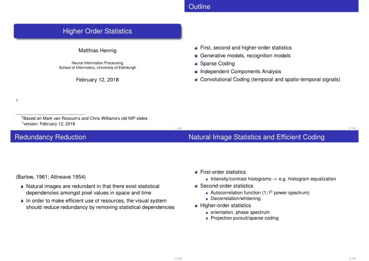
Outline Higher Order Statistics First, second and higher-order - PowerPoint PPT Presentation

Outline Higher Order Statistics First, second and higher-order statistics Matthias Hennig Generative models, recognition models Neural Information Processing Sparse Coding School of Informatics, University of Edinburgh Independent Components Analysis Convolutional Coding (temporal and spatio-temporal signals) February 12, 2018 1 0 Based on Mark van Rossum’s and Chris Williams’s old NIP slides 1 version: February 12, 2018 1 / 34 2 / 34 Redundancy Reduction Natural Image Statistics and Efficient Coding First-order statistics (Barlow, 1961; Attneave 1954) Intensity/contrast histograms ⇒ e.g. histogram equalization Second-order statistics Natural images are redundant in that there exist statistical Autocorrelation function (1 / f 2 power spectrum) dependencies amongst pixel values in space and time Decorrelation/whitening In order to make efficient use of resources, the visual system Higher-order statistics should reduce redundancy by removing statistical dependencies orientation, phase spectrum Projection pursuit/sparse coding 3 / 34 4 / 34

Image synthesis: First-order statistics Image synthesis: Second-order statistics [Figure: Olshausen, 2005] [Figure: Olshausen, 2005] Describe as correlated Gaussian statistics, or equivalently, power Log-normal distribution of intensities spectrum 5 / 34 6 / 34 Higher-order statistics Generative models, recognition models (§10.1, Dayan and Abbott) Left: observations. Middle: prior. Right: good model In image processing one would want, e.g. A are cars, B are faces. They would explain the image. [Figure: Olshausen, 2005] 7 / 34 8 / 34

Generative models, recognition models Examples of generative models Hidden (latent) variables h (causes) that explain visible variables u (e.g. image) Generative model (§10.1, Dayan and Abbott) � p ( u |G ) = p ( u | h , G ) p ( h |G ) Mixtures of Gaussians h Factor analysis, PCA Recognition model Sparse Coding p ( h | u , G ) = p ( u | h , G ) p ( h |G ) Independent Components Analysis p ( u |G ) Matching p ( u |G ) to the actual density p ( u ) . Maximize the log likelihood L ( G ) = � log p ( u |G ) � p ( u ) Train parameters G of the model using EM (expectation-maximization) 9 / 34 10 / 34 Sparse Coding Sparse Coding Area V1 is highly overcomplete. V1 : LGN ≈ 25:1 (in cat) Distributions that are close to zero most of the time but Firing rate distribution is typically exponential (i.e. sparse) occasionally far from 0 are called sparse Experimental evidence for sparse coding in insects, zebra finch, Sparse distributions are more likely than Gaussians to generate mouse, rabbit, rat, macaque monkey, human values near to zero, and also far from zero (heavy tailed) [Olshausen and Field, 2004] p ( x )( x − x ) 4 dx � kurtosis = � 2 − 3 �� p ( x )( x − x ) 2 dx ( Gaussian has kurtosis 0, positive k implies sparse distributions (super-Gaussian, leptokurtotic) Kurtosis is sensitive to outliers (i.e. it is not robust). See HHH §6.2 for other measures of sparsity Activity of a macaque IT cell in response to video images [Figure: Dayan and Abbott, 2001] 11 / 34 12 / 34

The sparse coding model Recognition step Single component model for image: u = g h . Suppose G is given. For given image, what is h ? Find g so that sparseness maximal, while � h � = 0, � h 2 � = 1. Multiple For g ( h ) corresponding to the Cauchy distribution, p ( h | u , G ) is components: difficult to compute exactly u = G h + n Olshausen and Field (1996) used MAP approximation Minimize [Olshausen and Field, 1996] N h E = [ reconstruction error ] − λ [ sparseness ] log p ( h | u , G ) = − 1 2 σ 2 | u − G h | 2 + � g ( h a ) + const Factorial: p ( h ) = � i p ( h i ) a = 1 Sparse: p ( h i ) ∝ exp( g ( h i )) (non-Gaussian) At maximum (differentiate w.r.t. to h ) Laplacian: g ( h ) = − α | h | Cauchy: g ( h ) = − log( β 2 + h 2 ) N h 1 n ∼ N ( 0 , σ 2 I ) � σ 2 [ u − G ˆ h ] b G ba + g ′ (ˆ h a ) = 0 Goal: find set of basis functions G such that the coefficients h are b = 1 as sparse and statistically independent as possible 1 σ 2 G T [ u − G ˆ h ] + g ′ (ˆ h ) = 0 or See D and A pp 378-383, and HHH §13.1.1-13.1.4 13 / 34 14 / 34 Learning of the model To solve this equation, follow dynamics N h dh a dt = 1 Now we have h , we can compare � [ u − G h ] b G ba + g ′ ( h a ) τ h σ 2 Log likelihood L ( G ) = � log p ( u |G ) � . Learning rule: b = 1 ∆ G ∝ ∂ L Neural network interpretation (notation, v = h ) Figure: Dayan and Abbott, 2001] ∂ G Basically linear regression (mean-square error cost) ∆ G = ǫ ( u − G ˆ h )ˆ h T Small values of h can be balanced by scaling up G . Hence b G 2 impose constraint on � ba for each cause a to encourage the variances of each h a to be approximately equal Dynamics does gradient ascent on log posterior. It is common to whiten the inputs before learning (so that � u � = 0 Note inhibitory lateral term and � uu T � = I ), to force the network to find structure beyond Process is guaranteed only to find a local (not global) maximum second order 15 / 34 16 / 34

Projective Fields and Receptive Fields Projective field for h a is G ba for all b values Note resemblance to simple cells in V1 Receptive fields: includes network interaction. Outputs of network are sparser than feedforward input, or pixel values Comparison with physiology: spatial-frequency bandwidth, orientation bandwidth [Figure: Dayan and Abbott (2001), after Olshausen and Field (1997)] 17 / 34 18 / 34 Gabor functions Can be used to model the receptive fields. A sinusoid modulated by a Gaussian envelope � � − x 2 − y 2 1 exp cos( kx − φ ) 2 πσ x σ y 2 σ 2 2 σ 2 x y Overcomplete: 200 basis functions from 12 × 12 patches [Figure: Olshausen, 2005] 19 / 34 20 / 34

Image synthesis: sparse coding ICA: Independent Components Analysis H ( h 1 , h 2 ) = H ( h 1 ) + H ( h 2 ) − I ( h 1 , h 2 ) Maximal entropy typically if I ( h 1 , h 2 ) = 0, i.e. P ( h 1 , h 2 ) = P ( h 1 ) P ( h 2 ) The more random variables are added, the more Gaussian. So look for the most non-Gaussian projection Often, but not always, this is most sparse projection. Can use ICA to de-mix (e.g. blind source separation of sounds) [Figure: Olshausen, 2005] 21 / 34 22 / 34 ICA derivation, [Bell and Sejnowski, 1995] ICA: Independent Components Analysis Derivation as generative model Linear network with output non-linearity v = W u , y j = f ( h j ) . Simplify sparse coding network, let G be square Find weight matrix maximizing information between u and y u = G h , W = G − 1 No noise (cf. Linsker), so I ( u , y ) = H ( y ) − H ( y | u ) = H ( y ) N h H ( y ) = � log p ( y ) � y = � log p ( u ) / det J � u with � p ( u ) = | det W | p h ([ W u ] a ) J ji = ∂ y j ∂ u i = ∂ h j ∂ y j � ∂ h j = w ij j f ′ ( h j ) ∂ u i a = 1 H ( y ) = log det W + � � j logf ′ ( h j ) � + const note Jacobian term Maximize entropy by producing a uniform distribution (histogram Log likelihood equalization: p ( h i ) = f ′ ( h i ) ). Choose f so that it encourages sparse p ( h ) , e.g. 1 / ( 1 + e − h ) . � � � L ( W ) = g ([ W u ] a ) + log | det W | + const det W helps to insure independent components a For f ( h ) = 1 / ( 1 + e − h ) , dH ( y ) / dW = ( W T ) − 1 + ( 1 − 2y ) x T See Dayan and Abbott pp 384-386 [also HHH ch 7] 23 / 34 24 / 34

Beyond Patches Stochastic gradient ascent gives update rule “Convolutional Coding” (Smith and Lewicki, 2005) ∆ W ab = ǫ ([ W − 1 ] ba + g ′ ( h a ) u b ) For a time series, we don’t want to chop the signal up into using ∂ log det W /∂ W ab = [ W − 1 ] ba arbitrary-length blocks and code those separately. Use the model Natural gradient update: multiply by W T W (which is positive M n m definite) to get � � h m i g m ( t − τ m u ( t ) = i ) + n ( t ) m = 1 i = 1 ∆ W ab = ǫ ( W ab + g ′ ( h a )[ h T W ] b ) τ m and h m are the temporal position and coefficient of the i th i i For image patches, again Gabor-like RFs are obtained instance of basis function g m In the ICA case PFs and RFs can be readily computed Notice this basis is M -times overcomplete 25 / 34 26 / 34 Want a sparse representation A signal is represented in terms of a set of discrete temporal events called a spike code , displayed as a spikegram Smith and Lewicki (2005) use matching pursuit (Mallat and Zhang, 1993) for inference Basis functions are gammatones (gamma modulated sinusoids), but can also be learned Zeiler et al (2010) use a similar idea to decompose images into sparse layers of feature activations. They used a Laplace prior on the h ’s. [Figure: Smith and Lewicki, NIPS 2004] 27 / 34 28 / 34