Image Processing I Computer Vision Fall 2018 Columbia University - PowerPoint PPT Presentation
Image Processing I Computer Vision Fall 2018 Columbia University Homework 1 Posted online today Due September 24 before class starts Turn in PDF and your code online Office Hours Carl: Monday 4:30pm to 5:30pm, CSB 502 Oscar:
Image Processing I Computer Vision Fall 2018 Columbia University
Homework 1 • Posted online today • Due September 24 before class starts • Turn in PDF and your code online
Office Hours • Carl: Monday 4:30pm to 5:30pm, CSB 502 • Oscar: Thursday 3-4pm, Mudd 500 • Xiaoning: Monday, 5-6pm, CS TA Room • Bo: Tuesday, 3-4pm, CS TA Room • James: Thursday 12-1pm, CS TA Room • Luc: Tuesday 4-5pm, CS TA Room
Image Formation Object Film Slide credit: Steve Seitz
Image Formation Object Barrier Film Add a barrier to block off most of the rays Slide credit: Steve Seitz
Image denoising Slide credit: S. Lazebnik
Average many photos! Time Slide credit: S. Lazebnik
What if just one? Slide credit: S. Lazebnik
Reminder: Images as Functions F [ x , y ]
Moving Average F [ x , y ] 0 0 0 0 0 0 0 0 0 0 0 0 0 0 0 0 0 0 0 0 0 0 0 90 90 90 90 90 0 0 0 0 0 90 90 90 90 90 0 0 0 0 0 90 90 90 90 90 0 0 0 0 0 90 0 90 90 90 0 0 0 0 0 90 90 90 90 90 0 0 0 0 0 0 0 0 0 0 0 0 0 0 90 0 0 0 0 0 0 0 0 0 0 0 0 0 0 0 0 0 Source: S. Seitz
Moving Average F [ x , y ] 0 0 0 0 0 0 0 0 0 0 0 0 0 0 0 0 0 0 0 0 0 0 0 0 90 90 90 90 90 0 0 0 0 0 90 90 90 90 90 0 0 0 0 0 90 90 90 90 90 0 0 0 0 0 90 0 90 90 90 0 0 0 0 0 90 90 90 90 90 0 0 0 0 0 0 0 0 0 0 0 0 0 0 90 0 0 0 0 0 0 0 0 0 0 0 0 0 0 0 0 0 Source: S. Seitz
Moving Average F [ x , y ] 0 0 0 0 0 0 0 0 0 0 0 0 0 0 0 0 0 0 0 0 0 10 0 0 0 90 90 90 90 90 0 0 0 0 0 90 90 90 90 90 0 0 0 0 0 90 90 90 90 90 0 0 0 0 0 90 0 90 90 90 0 0 0 0 0 90 90 90 90 90 0 0 0 0 0 0 0 0 0 0 0 0 0 0 90 0 0 0 0 0 0 0 0 0 0 0 0 0 0 0 0 0 Source: S. Seitz
Moving Average F [ x , y ] 0 0 0 0 0 0 0 0 0 0 0 0 0 0 0 0 0 0 0 0 0 10 20 0 0 0 90 90 90 90 90 0 0 0 0 0 90 90 90 90 90 0 0 0 0 0 90 90 90 90 90 0 0 0 0 0 90 0 90 90 90 0 0 0 0 0 90 90 90 90 90 0 0 0 0 0 0 0 0 0 0 0 0 0 0 90 0 0 0 0 0 0 0 0 0 0 0 0 0 0 0 0 0 Source: S. Seitz
Moving Average F [ x , y ] 0 0 0 0 0 0 0 0 0 0 0 0 0 0 0 0 0 0 0 0 0 10 20 30 0 0 0 90 90 90 90 90 0 0 0 0 0 90 90 90 90 90 0 0 0 0 0 90 90 90 90 90 0 0 0 0 0 90 0 90 90 90 0 0 0 0 0 90 90 90 90 90 0 0 0 0 0 0 0 0 0 0 0 0 0 0 90 0 0 0 0 0 0 0 0 0 0 0 0 0 0 0 0 0 Source: S. Seitz
Moving Average F [ x , y ] 0 0 0 0 0 0 0 0 0 0 0 0 0 0 0 0 0 0 0 0 0 10 20 30 0 0 0 90 90 90 90 90 0 0 0 0 0 90 90 90 90 90 0 0 0 0 0 90 90 90 90 90 0 0 ? 0 0 0 90 0 90 90 90 0 0 0 0 0 90 90 90 90 90 0 0 0 0 0 0 0 0 0 0 0 0 0 0 90 0 0 0 0 0 0 0 0 0 0 0 0 0 0 0 0 0 Source: S. Seitz
Moving Average F [ x , y ] 0 0 0 0 0 0 0 0 0 0 0 0 0 0 0 0 0 0 0 0 0 10 20 30 30 30 20 10 0 0 0 90 90 90 90 90 0 0 0 20 40 60 60 60 40 20 0 0 0 90 90 90 90 90 0 0 0 30 60 90 90 90 60 30 0 0 0 90 90 90 90 90 0 0 0 30 50 80 80 90 60 30 0 0 0 90 0 90 90 90 0 0 0 30 50 80 80 90 60 30 0 0 0 90 90 90 90 90 0 0 0 20 30 50 50 60 40 20 0 0 0 0 0 0 0 0 0 0 10 20 30 30 30 30 20 10 0 0 90 0 0 0 0 0 0 0 10 10 10 0 0 0 0 0 0 0 0 0 0 0 0 0 0 0 Source: S. Seitz
Filtering Filter Output Image Input Image We want to remove unwanted sources of variation, and keep the information relevant for whatever task we need to solve Source: Bill Freeman
Linear Filtering Filter Output Image Input Image For a filter to be linear, it must satisfy two properties: • filter(im, f1 + f2) = filter(im, f1) + filter(im, f2) • C * filter(im, f1) = filter(im, C * f1) Source: Bill Freeman
Convolution F [ x , y ] 0 0 0 0 0 0 0 0 0 0 G [ x , y ] 0 0 0 0 0 0 0 0 0 0 0 10 20 30 30 30 20 10 0 0 0 90 90 90 90 90 0 0 0 20 40 60 60 60 40 20 = 0 0 0 90 90 90 90 90 0 0 1 1 1 0 30 60 90 90 90 60 30 1 * 0 0 0 90 90 90 90 90 0 0 0 30 50 80 80 90 60 30 1 1 1 0 0 0 90 0 90 90 90 0 0 0 30 50 80 80 90 60 30 9 1 1 1 0 0 0 90 90 90 90 90 0 0 0 20 30 50 50 60 40 20 0 0 0 0 0 0 0 0 0 0 10 20 30 30 30 30 20 10 0 0 90 0 0 0 0 0 0 0 10 10 10 0 0 0 0 0 0 0 0 0 0 0 0 0 0 0
Convolution • Let f be an image/function, and g is the kernel/filter • The convolution is defined as: ( f * g )[ x , y ] = ∑ f [ x − i , y − j ] g [ i , j ] i , j
Convolution ( f * g )[ x , y ] = ∑ f [ x − i , y − j ] g [ i , j ] i , j g f
Convolution ( f * g )[ x , y ] = ∑ f [ x − i , y − j ] g [ i , j ] i , j g Flip LR, UD f
Convolution Practice 0 0 0 ? 0 1 0 0 0 0 Source: D. Lowe
Convolution Practice 0 0 0 0 1 0 0 0 0 Source: D. Lowe
Convolution Practice 0 0 0 ? 0 0 1 0 0 0 Source: D. Lowe
Convolution Practice Translation Filter 0 0 0 0 0 1 0 0 0 Source: D. Lowe
Convolution Practice 1 1 1 ? 1 1 1 1 9 1 1 1 Source: D. Lowe
Convolution Practice Blur Filter 1 1 1 1 1 1 1 9 1 1 1 Source: D. Lowe
Convolution Practice ? Source: D. Lowe
Convolution Practice 0 0 0 1 1 1 ? − 1 0 2 0 1 1 1 9 0 0 0 1 1 1 Source: D. Lowe
Convolution Practice Sharpening Filter 0 0 0 1 1 1 − 1 0 2 0 1 1 1 9 0 0 0 1 1 1 Source: D. Lowe
Sharpening Source: D. Lowe
Sharpening - = Image Blurred Detail + = Image Detail Sharpened
Convolution Properties Commutative: F ∗ H = H ∗ F Associative: ( F ∗ H ) ∗ G = F ∗ ( H ∗ G ) Distributive: ( F ∗ G ) + ( H ∗ G ) = ( F + H ) ∗ G
Convolution Properties Scale: filter(A * f) = A * filter(f) Shift Invariance: filter(shift(f)) = shift(filter(f))
Cross-Correlation • Conceptually simpler, but not as nice properties: ( f * g )[ x , y ] = ∑ f [ x + i , y + j ] g [ i , j ] i , j g f
Boundary Issues full same valid g g g g g g f f f g g g g g g Slide credit: S. Lazebnik
Border Padding Zero Pad Circular Replicate Symmetric
Box Filter
Gaussian Filter
Gaussian Filter 0.003 0.013 0.022 0.013 0.003 0.013 0.059 0.097 0.059 0.013 0.022 0.097 0.159 0.097 0.022 0.013 0.059 0.097 0.059 0.013 0.003 0.013 0.022 0.013 0.003 5 x 5, σ = 1 Constant factor at front makes volume sum to unity Source: C. Rasmussen
Standard Deviation σ = 2 with σ = 5 with 30 x 30 30 x 30 kernel kernel Standard deviation σ : determines extent of smoothing Source: K Grauman
Changing Sigma
Kernel Width The Gaussian function has infinite support, but discrete filters use finite kernels Rule of thumb: set filter half-width to about 3 σ Source: K Grauman
Complexity What is the complexity of filtering an n × n image with an m × m kernel?
Complexity What is the complexity of filtering an n × n image with an m × m kernel? O(n 2 m 2 )
Separable Convolution Two dimensional Gaussian is product of two Gaussians: 2 πσ 2 exp ( − x 2 + y 2 ) 1 G ( x , y ) = 2 σ 2 exp ( − x 2 exp ( − y 2 2 σ 2 ) 2 σ 2 ) 1 1 = 2 πσ 2 πσ Take advantage of associativity: f = f * * *
Complexity What is the complexity of filtering an n × n image with an m × m kernel? O(n 2 m 2 ) What if kernel is separable?
Complexity What is the complexity of filtering an n × n image with an m × m kernel? O(n 2 m 2 ) What if kernel is separable? O(n 2 m)
Denoising Additive Gaussian Noise Gaussian Filter (sigma=1)
What’s wrong? Salt and Pepper Noise Gaussian Filter (sigma=1)
Median Filter • A median filter operates over a window by selecting the median intensity in the window Is median filtering linear? Source: Kristen Grauman
Why use median? Source: Kristen Grauman
What’s wrong? Salt and Pepper Noise Median Filter 3x3
Median Filtering Median 3x3 Median 5x5 Median 9x9
Image Gradients
Image Gradients How does intensity change as you move left to right? How do you take the derivative of an image?
First Derivative ∂ I * [ − 1,1] = ∂ x ∂ I * [ − 1,1] T = ∂ y
Second Derivative ∂ 2 I * [ − 1,1] = ∂ x 2 ∂ 2 I * [ − 1,1] T = ∂ y 2
Image Gradients Source: Seitz and Szeliski
What causes an edge? Source: G Hager
What causes an edge? Surface normal discontinuities Source: G Hager
What causes an edge? Boundaries of material properties Source: G Hager
What causes an edge? Boundaries of material properties Source: G Hager
What causes an edge? Boundaries of lighting Source: G Hager
Edge Types Source: G Hager
What is an edge? Source: G Hager
What about noise? Source: G Hager
Recommend
More recommend
Explore More Topics
Stay informed with curated content and fresh updates.


![CCD Image Processing: CCD Image Processing: [ ] [ ] r x y , d x y , Raw File [ ]](https://c.sambuz.com/775303/ccd-image-processing-ccd-image-processing-s.webp)
