Image Definition and point operation g p p WHAT IS AN IMAGE? - PowerPoint PPT Presentation
VIDEO SIGNALS VIDEO SIGNALS Image Definition and point operation g p p WHAT IS AN IMAGE? WHAT IS AN IMAGE? Ideally, we think of an image Id ll hi k f i i mage as a 2-di 2 di di dimens mensiona i onal l li l li li h light
VIDEO SIGNALS VIDEO SIGNALS Image Definition and point operation g p p
WHAT IS AN IMAGE? WHAT IS AN IMAGE? Ideally, we think of an image Id ll hi k f i i mage as a 2-di 2 di di dimens mensiona i onal l li l li li h light int intensity function ity function, f(x,y) , where x and y are spatial coordinates, and f at (x,y) is related to the brightness or , ( ,y) g color of the image at that point. In practice, most images are defined over a rectangle. Continuous in amplitude („continuous-tone“) C ti i lit d ( ti t “) Continuous in space: no pixels!
DIGITAL IMAGES AND PIXELS DIGITAL IMAGES AND PIXELS A digit A digit digit l i digital i l ima i mage i g i i th is th th the represen representati t ti tion on of f f a con f conti tinuous ti ti nuous image image f(x,y) by a 2-d array of discrete samples. The amplitude of each sample is quantized to be amplitude of each sample is quantized to be represented by a finite number of bits. Each element of the 2-d array of samples is called a Each element of the 2 d array of samples is called a pix pixel l or pel pel (fr from “picture element”) om “picture element”) Pixels are point samples, without extent. p p , A pixel is not: Round, square, or rectangular ou d, squa e, o ecta gu a An element of an image sensor m An element of a display
A DIGITAL IMAGE IS REPRESENTED BY NUMBERS A DIGITAL IMAGE IS REPRESENTED BY NUMBERS
AN IMAGE CAN BE REPRESENTED AS A MATRIX AN IMAGE CAN BE REPRESENTED AS A MATRIX The pixel values f(x,y) are sorted into the matrix in „natural“ Th i l l f( ) t d i t th t i i t l“ order, with x corresponding to the column and y to the row index index. Matlab, instead, uses matrix convention. This results in f(x,y) = f yx , where f yx denotes an individual element in common matrix f yx , where f yx denotes an individual element in common matrix notation. For a color image, f g f might be one of the components. g p
IMAGE SIZE AND RESOLUTION IMAGE SIZE AND RESOLUTION These images were produced by simply picking every n - th sample horizontally and vertically y p y y and replicating that value n x n times. We can do better prefiltering before subsampling to avoid aliasing Smooth interpolation
IMAGE OF DIFFERENT SIZE IMAGE OF DIFFERENT SIZE
FEWER PIXELS MEAN LOWER SPATIAL RESOLUTION
COLOR COMPONENTS COLOR COMPONENTS
DIFFERENT NUMBERS OF GRAY LEVELS DIFFERENT NUMBERS OF GRAY LEVELS
HOW MANY GRAY LEVELS ARE REQUIRED? HOW MANY GRAY LEVELS ARE REQUIRED? How many gray levels are required? ? Digital images typically are quantized to 256 gray levels.
STORAGE REQUIREMENTS FOR DIGITAL IMAGES STORAGE REQUIREMENTS FOR DIGITAL IMAGES Image LxN pixels 2 B gray levels c color Image LxN pixels, 2 B gray levels, c color components Size = L x N x B x c Size = L x N x B x c Example: L=N=512 B=8 c=1 (i e monochrome) Size Example: L=N=512, B=8, c=1 (i.e., monochrome) Size = 2,097,152 bits (or 256 kByte) Example: LxN=1024x1280, B=8, c=3 (24 bit RGB p 0 0, , ( image) Size = 31,457,280 bits (or 3.75 MByte) Much less with (lossy) compression! For a video multiply by the frame rate and by the number of seconds of its lenght.
BRIGHTNESS DISCRIMINATION EXPERIMENT BRIGHTNESS DISCRIMINATION EXPERIMENT Can you see the circle? C h i l ? Visibility threshold
CONTRAST WITH 8 BIT CONTRAST WITH 8 BIT CONTRAST WITH 8 BITS A CONTRAST WITH 8 BITS A ACCORDING T ACCORDING T CCORDING TO WEBER CCORDING TO WEBER WEBER‘S LA WEBER S LA S LAW LAW Assume that the luminance difference between two successive A th t th l i diff b t t i representative levels is just at visibility threshold For Typical display contrast Cathode ray tube 100:1 Cathode ray tube 100:1 Print on paper 10:1 Suggests uniform quantization in the log( I) domain
MOST COMMON POINT OPERATIONS ON IMAGES MOST COMMON POINT OPERATIONS ON IMAGES Intensity scaling Brightness/Contrast adjustment Brightness/Contrast adjustment Gamma adjustment Histogram equalization Image averaging Image averaging High-dynamic range from multiple exposures Image subtraction
HISTOGRAMS HISTOGRAMS Distribution of gray levels can be judged by measuring a histogram: Distribution of gray-levels can be judged by measuring a histogram: For B-bit image, initialize 2 B counters with 0 Loop over all pixels x,y When encountering gray level f(x,y)=i, increment counter #i Histogram can be interpreted as an estimate of the probability density function ( pdf ) of an underlying random process. You can also use fewer, larger bins to trade off amplitude resolution against sample size.
EXAMPLE HISTOGRAM EXAMPLE HISTOGRAM
EXAMPLE HISTOGRAM EXAMPLE HISTOGRAM
HISTOGRAM COMPARISON HISTOGRAM COMPARISON Both these images present the same Histogram
HISTOGRAM COMPARISON HISTOGRAM COMPARISON Histogram as an invariant feature
HISTOGRAM COMPARISON HISTOGRAM COMPARISON
HISTOGRAM EQUALIZATION HISTOGRAM EQUALIZATION Idea: find a non linear transformation Idea: find a non-linear transformation g g = = T ( f ) to be applied to each pixel of the input image f(x,y) f(x,y), such that a uniform distribution of gray levels in the entire range results for the if di t ib ti f l l i th ti lt f th output image g(x,y). g(x,y). Analyze ideal, continuous case first, assuming 0 0 ≤ f f ≤ 1 1 0 0 ≤ g g ≤ 1 T(f) T(f) is strictly monotonically increasing, hence, there exists f = T f = T − 1 (g) (g) 0 0 ≤ g g ≤ 1 Goal: pdf (probability density function) p g (g) Goal: pdf (probability density function) p g (g) (g) = cons (g) cons const. over the range const. over the range
HISTOGRAM EQUALIZATION FOR CONTINUOUS CASE CONTINUOUS CASE From basic probability theory Consider the transformation function Then
HISTOGRAM EQUALIZATION FOR CONTINUOUS CASE
HISTOGRAM EQUALIZATION FOR DISCRETE CASE Now, f only assumes discrete amplitude values f 0 , f 1 , …,f L-1 , with probabilities: Discrete approximation of The resulting values g k are in the range [0,1] and need to be scaled and rounded appropriately rounded appropriately
HISTOGRAM EQUALIZATION EXAMPLE HISTOGRAM EQUALIZATION EXAMPLE
HISTOGRAM EQUALIZATION EXAMPLE HISTOGRAM EQUALIZATION EXAMPLE
HISTOGRAM EQUALIZATION EXAMPLE HISTOGRAM EQUALIZATION EXAMPLE
HISTOGRAM EQUALIZATION EXAMPLE HISTOGRAM EQUALIZATION EXAMPLE
ADAPTIVE HISTOGRAM EQUALIZATION ADAPTIVE HISTOGRAM EQUALIZATION Apply histogram equalization based on a histogram obtained from a portion of the image Must limit contrast expansion in flat regions of the image, e.g. by clipping individual histogram the image, e.g. by clipping individual histogram values to a maximum
ADAPTIVE HISTOGRAM EQUALIZATION ADAPTIVE HISTOGRAM EQUALIZATION
ADAPTIVE HISTOGRAM EQUALIZATION ADAPTIVE HISTOGRAM EQUALIZATION
POINT OPERATIONS BETWEEN IMAGES POINT OPERATIONS BETWEEN IMAGES Image averaging for noise reduction Combination of different exposure for high- Combination of different exposure for high dynamic range imaging Image subtraction for change detection I g bt ti f h g d t ti Accurat ccurate ali alignment is g g nment is alw always a y y s a re requirement q uirement
IMAGE AVERAGING FOR NOISE REDUCTION IMAGE AVERAGING FOR NOISE REDUCTION
IMAGE AVERAGING FOR NOISE REDUCTION IMAGE AVERAGING FOR NOISE REDUCTION Take N aligned images T k N li d i Average Image: A I Mean squared error vs. noise-free image g
HIGH DYNAMIC RANGE IMAGING HIGH-DYNAMIC RANGE IMAGING 16 exposures, one f-stop (2X) apart
IMAGE SUBTRACTION IMAGE SUBTRACTION Find differences/changes Find differences/changes between 2 mostly identical images Example from IC f C manufacturing: defect detection in photomasks detection in photomasks by die-to-die comparison
WHERE IS THE DEFECT? WHERE IS THE DEFECT? Image A without defect Image B with defect
ABSOLUTE DIFFERENCE BETWEEN TWO IMAGES ABSOLUTE DIFFERENCE BETWEEN TWO IMAGES Without alignment With Alignment
DIGITAL SUBTRACTION ANGIOGRAPHY DIGITAL SUBTRACTION ANGIOGRAPHY
Recommend
More recommend
Explore More Topics
Stay informed with curated content and fresh updates.
