How to use Statas sem with small samples? New corrections for the - PowerPoint PPT Presentation
How to use Statas sem with small samples? New corrections for the L. R. 2 statistics and fit indices Meeting of the German Stata User Group at the Konstanz University, June 22nd, 2018 ? All models are false, but some are useful.
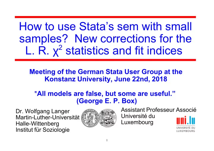
How to use Stata’s sem with small samples? New corrections for the L. R. χ 2 statistics and fit indices Meeting of the German Stata User Group at the Konstanz University, June 22nd, 2018 ? All models are false, but some are useful.” (George E. P. Box) Assistant Professeur Associé Dr. Wolfgang Langer Université du Martin-Luther-Universität Luxembourg Halle-Wittenberg Institut für Soziologie 1
Contents What is the problem? What are the solutions for it? What do we know from Monte-Carlo simulation studies? How to implement it in Stata? Empirical example of Islamophobia in Germany 2016 Conclusions 2
What is the problem? In empirical research more and more people estimate their SEM using a small sample (n<100) in psychology, marketing or business research When working with small samples we are confronted with a severe problem < The traditional Likelihood-Ratio χ 2 goodness-of-fit test and all fit-indices basing on it tend to overreject acceptable models. They are too conservative! < This is caused by the pure approximation of the χ 2 test statistics to the noncentral χ 2 distribution 3
What are solutions for it? Several correction procedures have been developed to improve the approximation of the L.R.χ 2 -test statistics (T ML ) to the noncentral χ 2 distribution < The Bartlett correction < The Yuan correction < The Swain correction 4
The Bartlett correction Bartlett developed a small-sample correction to test the exact fit of exploratory factor models (1937, 1950, 1954) estimated by ML 4 2 5 k p 1 b 6 n Bartlett corrected T b T MLb ML : Legend : number of latent variables factors k : number of observed variables (indicators) p : sample size +1 n N 5
The Yuan correction Yuan (2005) proposed an ? ad hoc” simplifi- cation of a Bartlett like correction formula developed by Wakaki, Eguchi & Fujikoshi (1990) for covariance structure models 2 2 7 k p 1 y 6 n Yuan corrected T y T MLy ML 6
The Swain correction Swain (1975) proposed the following correction of the test statistics T ML 2 2 2 3 1 2 3 1 p p p q q q 1 s 12 d n 1 4 1 8 1 p p d with q 2 Swain corrected T s T MLs ML : Legend : number of observed variables(indicators) p : degreesof freedomof actualmodel d n : samplesize 1 N 7
What do we know from M. C. studies? A lot of Monte-Carlo simulation studies with small samples have been made to evaluate the shown corrections. They test systematically < Violations of the multivariate normal distribution assumption < Sample size < Number of indicators < Extend of model misspecification 8
What do we know ... ? Fouladi (2000) and Newitt & Hancock (2004) recommended the Bartlett correction of the T ML for normal data. For not normal distributed data they proposed the Bartlett correction of the Satorra-Bentler adjusted T ML Herzog, Boomsma & Reinecke (2007) and Herzog & Boomsma (2009/13) showed that < Both Bartlett and Yuan corrections overestimate the type-I-error rate when sample size decreases < The Swain correction is the winner for small sample sizes and large models with many indicators – It reduces to a high extend the type-I-error rate – It works even to a sample size to estimated parameter ratio of 2:1 9
What do we know ... ? Herzog, Boomsma & Reinecke (2007) and Herzog & Boomsma (2009/13) also developed and tested a modified version of Tucker-Lewis- Index (TLI or NNFI) using the Swain-rescaled T ML for the target model and usual T ML for the baseline model < It clearly outperforms the TLI calculated by standard programs like MPLUS, EQS, LISREL < It reports correctly the misspecification of the SEM < They recommended this correction also for the Comparativ Fit Index developed by Bentler (1990) and Steiger’s Root-Mean-Squared-Error of Approximation (RMSEA) 10
Swain corrected Tucker-Lewis Index For normal distributed data: Formulas T s T ML ML bs ms df df bs ms TLI T ML 1 bs df bs For not normal distributed data: sb T s sb T ML ML bs ms df df bs ms TLI sb T ML 1 bs df bs 11
Swain corrected Comparative-Fit Index Formulas For normal distributed data: T df s T df M L bs M L ms bs ms CFI T df M L bs bs For not normal distributed data: sb T df s sb T df M L bs M L ms bs ms CFI sb T df M L bs bs 12
Swain corrected RMSEA Formulas For normal distributeddata: s T df ML ms RMSEA ms n df ms For not normaldistributeddata: s sb T df ML ms RMSEA ms n df ms 13
How to implement it in Stata ? In 2013 John Antonakis and Nicolas Bastardoz, both from University of Lausanne, Switzerland, published their ? swain.ado” calculating only the Swain-corrected T ML value for comparison of the actual vs. saturated model I have modified this ado-file calculating now Swain-corrected T ML , TLI, CFI and RMSEA – Under the assumption of multivariate normality (Jöreskog 1970, p. 239) – Under violation of the multivariate normality assumption (not normal distributed data) using the Satorra-Bentler-corrected T ML – All calculated scalars are displayed and returned in r-containers 14
Empirical example of Islamophobia SEM explaining Islamophobia in West Germany 2016 5% sample of the German General Social Survey 2016, subsample west: n=84 Presentation of used indicators Test of multivariate normal distribution of observed indicators (mvtest in Stata) Estimated results from sembuilder Results of estat gof, stats(all) Output of my swain_gof.ado 15
SEM to explain Islamophobia e e e 13 mm01 e 11 12 2 0 id02 educ2 incc mm02r e 3 0 0 0 0 e 1 mm03 e 4 0 SES Islamophob mm04 e 5 e 0 8 mm05r e 6 pa01 Authoritu 0 mm06 e 7 0 lp01 lp02 0 0 e e 9 10 16
Used indicators Factor SES: Socio-economic status < id02: Self rating of social class – Underclass to upperclass [1;5] < educ2: educational degree – Without degree to grammar school [1;5] < incc: income class (quintiles) [1;5] Factor Authoritu: authoritarian submission < lp01: Thank to the leading heads saying us what to do [1;7] < lp02: It is good for a child to learn to obey its parents [1;7] Single indicator pa01: left-right self-rating < 1) left .. 10) right 17
Used indicators Factor Islamophobia < Six items [1;7] – mm01 The religious practice of Islam should be restricted in Germany – mm02r The Islam does not belong to Germany – mm03 The presence of Muslims leads to conflicts – mm04 The Islamic communities should be supervised by the state – mm05r I object to have an Islamic mayor in my town – mm06 There are a lot of religious fanatics in the Islamic community 18
Test of multivariate normality (n = 84) . mvtest normality mm01 mm02r mm03 mm04 mm05r mm06 lp01 lp02 pa01 id02 educ2 incc, uni stats(all) Test for univariate normality joint Variable Pr(Skewness) Pr(Kurtosis) adj chi2(2) Prob>chi2 mm01 0.4475 0.0000 44.17 0.0000 Except id02 all mm02r 0.0086 0.4302 6.91 0.0317 indicators violate the mm03 0.4600 0.0040 7.89 0.0194 assumption of mm04 0.1012 0.0002 13.43 0.0012 mm05r 0.4737 0.0000 . 0.0000 univariate nomality! mm06 0.5839 0.0000 24.28 0.0000 lp01 0.1037 0.0827 5.47 0.0648 lp02 0.0000 0.0174 19.23 0.0001 pa01 0.0280 0.9034 4.83 0.0893 id02 0.9191 0.4762 0.53 0.7685 educ2 0.0255 0.0142 9.47 0.0088 incc 0.8780 0.0000 20.93 0.0000 All together violate the assumption of Test for multivariate normality multivariate normality! Mardia mSkewness = 31.04157 chi2(364) = 452.560 Prob>chi2 = 0.0011 Mardia mKurtosis = 173.1796 chi2(1) = 1.677 Prob>chi2 = 0.1954 Henze-Zirkler = 1.034168 chi2(1) = 40.558 Prob>chi2 = 0.0000 Doornik-Hansen chi2(24) = 118.558 Prob>chi2 = 0.0000 19
Standardized solution of the SEM with Satorra-Bentler corrections: vce(sbentler) e e e 11 0.39 0.67 0.85 mm01 e 0.59 12 13 2 0 id02 educ2 incc mm02r e 0.57 0.63 3 0 0 0 0 e 1 0.78 0.57 0.39 mm03 e 0.72 4 0 SES Islamophob 1 0.25 mm04 e 0.39 -0.66 5 -0.04 e 0 8 0.61 mm05r e 0.65 pa01 6 Authoritu 0.53 0 1 Sample size: N = 84 0.39 mm06 e 0.38 0.59 R 2 (Islamophobia) = 0.3716 7 0 R 2 (Authoritu) = 0.7463 lp01 lp02 TLI_SB = 0.897 0 0 CFI_SB = 0.921 N:t = 84 : 27 . 3:1 e e RMSEA_SB = 0.059 0.86 0.85 9 10 20
Recommend
More recommend
Explore More Topics
Stay informed with curated content and fresh updates.













![-Samples [AB98] Hyp: domain S is a smooth curve or surface. S 1 -Samples [AB98] Hyp:](https://c.sambuz.com/966627/samples-s.webp)
