How to Solve Complex Problems in Parallel (Parallel Divide and - PowerPoint PPT Presentation
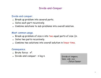
How to Solve Complex Problems in Parallel (Parallel Divide and Conquer and Task Parallelism) Kenjiro Taura 1 / 97 Contents 1 Introduction 2 An example : k -d tree construction k -d tree 3 Parallelizing divide and conquer algorithms Basics
Parallelizing divide and conquer Divide and conquer algorithms are easy to parallelize if the programming language/library supports asynchronous recursive calls ( task parallel systems) OpenMP task constructs Intel Threading Building Block (TBB) Cilk, CilkPlus we use TBB in the following because of its performance portability T0 T1 T161 T2 T40 T162 T184 T3 T31 T41 T77 T163 T172 T185 T187 T4 T29 T32 T38 T42 T66 T78 T102 T164 T166 T173 T175 T186 T188 T190 T5 T11 T30 T33 T37 T39 T43 T62 T67 T74 T79 T82 T103 T153 T165 T167 T171 T174 T176 T181 T189 T191 T6 T7 T12 T24 T34 T35 T44 T63 T65 T68 T72 T75 T76 T80 T81 T83 T101 T104 T122 T154 T155 T168 T169 T177 T179 T182 T192 T8 T9 T13 T14 T25 T26 T36 T45 T61 T64 T69 T71 T73 T84 T93 T105 T120 T123 T137 T156 T158 T170 T178 T180 T183 T193 T195 T10 T15 T23 T27 T46 T60 T70 T85 T94 T106 T111 T121 T124 T128 T138 T152 T157 T159 T160 T194 T196 T198 T16 T20 T28 T47 T56 T86 T87 T95 T96 T107 T110 T112 T114 T125 T129 T135 T139 T143 T197 T199 T17 T21 T48 T57 T88 T92 T97 T108 T109 T113 T115 T117 T126 T130 T136 T140 T144 T146 T18 T22 T49 T55 T58 T89 T90 T98 T100 T116 T118 T127 T131 T141 T145 T147 T150 T19 T50 T54 T59 T91 T99 T119 T132 T134 T142 T148 T149 T151 T51 T53 T133 19 / 97 T52
Parallelizing k -d tree construction with tasks it’s as simple as doing two recursions in parallel! e.g., with OpenMP tasks ✞ build(P, R, depth) { 1 if (|P| == 0) { 2 return 0; / ∗ empty ∗ / 3 } else if (|P| <= threshold) { 4 return make_leaf(P, R, depth); 5 } else { 6 s = find_median(P, depth % D); 7 R0,R1 = split_rect(R, depth % D, s.pos[depth % D]); 8 P0,P1 = partition(P - { p }, depth % D, s.pos[depth % D]); 9 #pragma omp task shared(n0) 10 n0 = build(P0, R0, depth + 1); 11 #pragma omp task shared(n1) 12 n1 = build(P1, R1, depth + 1); 13 #pragma omp taskwait 14 return make_node(p, n0, n1, depth); 15 } 16 } 17 do you want to parallelize it with only parallel loops? 20 / 97
Contents 1 Introduction 2 An example : k -d tree construction k -d tree 3 Parallelizing divide and conquer algorithms Basics Intel TBB 4 Reasoning about speedup Work and critical path length Greedy scheduler theorem Calculating work and critical path 5 More divide and conquer examples Merge sort Cholesky factorization Triangular solve Matrix multiply 21 / 97
Task parallelism in Intel TBB we use Intel TBB as a specific example of task parallel systems, primarily because of its compiler-independence consider executing the following two calls in parallel ✞ n0 = build(P0, R0, depth + 1); 1 n1 = build(P1, R1, depth + 1); 2 in TBB, this can be expressed by: ✞ tbb::task group tg; 1 tg.run([&] { n0 = build(P0, R0, depth + 1); } ); 2 n1 = build(P1, R1, depth + 1); 3 tg.wait(); 4 note: you can, but do not have to, create a task for the second recursion 22 / 97
Parallelizing k -d tree construction with TBB ✞ build(P, R, depth) { 1 if (|P| == 0) { 2 return 0; / ∗ empty ∗ / 3 } else if (|P| <= threshold) { 4 return make_leaf(P, R, depth); 5 } else { 6 s = find_median(P, depth % D); 7 R0,R1 = split_rect(R, depth % D, s.pos[depth % D]); 8 P0,P1 = partition(P - { p }, depth % D, s.pos[depth % D]); 9 tbb::task group tg; 10 tg.run([&] { n0 = build(P0, R0, depth + 1); } ); 11 n1 = build(P1, R1, depth + 1); 12 tg.wait(); 13 return make_node(p, n0, n1, depth); 14 } 15 } 16 23 / 97
A summary of task group class in TBB include <tbb/task group.h> create an instance of tbb::task group class prior to creating tasks task group::run( c ) method: creates a task that executes c () c is any callable object task group::wait() method: waits for the completion of all tasks that are run ’ed by the task group object 24 / 97
How TBB executes tasks? details are complex and will be covered later, but the following suffices for now as an cores (threads representing cores) approximation it globally pools ready (runnable) tasks somewhere from which cores fetch and execute tasks tasks can be executed by any core (load balancing) tasks each core tries to fill it with tasks as much as possible (greedy) 25 / 97
A note on callable and C++ lambda expression any callable object can be passed to run method a callable object is an object defining operator() e.g. ✞ class my_task { 1 int x; 2 my_task(int arg) { x = arg; } 3 void operator() () { print(x); } 4 } 5 ✞ tbb::task_group tg; 1 my_task c(3); 2 tg.run(c); 3 26 / 97
C++ lambda expression (closure) it is cumbersome to manually define a class for each task creation; C++ lambda expression reduces this labor not specific to TBB, but a recent extension to C++ (C++0x, C++11) that TBB programmers would appreciate syntax in brief: [ capture-list ] { statements } this represents a callable object that, when called, executes statements . capture-list specifies which variables to copy into the closure, and which variables to share between the closure and the outer context 27 / 97
C++ lambda expression examples (1) copy everything ( x and y ); ✞ int x = 3; 1 C = [=] { print(x); }; 2 x = 4; 3 C(); // will print 3, not 4 4 share everything ✞ int x = 3; 1 C = [&] { print(x); }; 2 x = 4; 3 C(); // will print 4, not 3 4 28 / 97
C++ lambda expression examples (2) share specific variables ✞ int z; 1 C = [=,&z] { z = 4; }; 2 C(); 3 print(z); // will print 4, not 3 4 you will (often) like to share large arrays to avoid large copies ✞ int a[1000]; 1 C = [=,&a] { gemm(a) }; 2 C(); 3 29 / 97
Which variables to share/copy when you run ? if you want to get a return value, do not forget to share the receiving variable presumably wrong ✞ tg.run([=] { y = f(x); }); 1 you should insead write: ✞ tg.run([=,&y] { y = f(x); }); 1 make sure arguments you passed to the task are not overwritten by the parent presumably wrong ✞ for (i = 0; i < n; i++) { 1 tg.run([&] { y = f(i); }); 2 } 3 you should insead write: ✞ tg.run([&,=i] { y = f(i); }); 1 30 / 97
Contents 1 Introduction 2 An example : k -d tree construction k -d tree 3 Parallelizing divide and conquer algorithms Basics Intel TBB 4 Reasoning about speedup Work and critical path length Greedy scheduler theorem Calculating work and critical path 5 More divide and conquer examples Merge sort Cholesky factorization Triangular solve Matrix multiply 31 / 97
Reasoning about speedup so you parallelized your program, you now hope to get some speedup on parallel machines! 32 / 97
Reasoning about speedup so you parallelized your program, you now hope to get some speedup on parallel machines! PROBLEM: how to reason about the execution time (thus speedup) of the program with P processors 32 / 97
Reasoning about speedup so you parallelized your program, you now hope to get some speedup on parallel machines! PROBLEM: how to reason about the execution time (thus speedup) of the program with P processors ANSWER: get the work and the critical path length of the computation 32 / 97
Contents 1 Introduction 2 An example : k -d tree construction k -d tree 3 Parallelizing divide and conquer algorithms Basics Intel TBB 4 Reasoning about speedup Work and critical path length Greedy scheduler theorem Calculating work and critical path 5 More divide and conquer examples Merge sort Cholesky factorization Triangular solve Matrix multiply 33 / 97
Work and critical path length Work: = the total amount of work of the computation = the time it takes in a serial execution Critical path length: = the maximum length of dependent chain of computation a more precise definition follows, with computational DAGs 34 / 97
Computational DAGs The DAG of a computation is a directed acyclic graph in which: ✞ main() { 1 a node = an interval of computation A(); 2 create_task B(); 3 free of task parallel primitives C(); 4 wait(); // wait for B i.e. a node starts and ends by a task 5 D(); 6 parallel primitive } 7 we assume a single node is executed non-preemptively an edge = a dependency between two A nodes, of three types: create task parent → created child child → waiting parent B C wait a node → the next node in the same end task task D 35 / 97
A computational DAG and critical path length Consider each node is augmented with a time for a processor to execute it A create task ( the node’s execution time ) Define the length of a path to be the sum of execution time of the nodes on B C wait the path end task D Given a computational DAG, critical path length = the length of the longest paths from the start node to the end node in the DAG (we often say critical path to in fact mean its length) 36 / 97
A computational DAG and work Work, too, can be elegantly defined in light of computational DAGs A create task B C wait end task D Given a computational DAG, work = the sum of lengths of all nodes 37 / 97
What do they intuitively mean? A create task The critical path length represents the B C “ideal” execution time with infinitely wait end task many processors D i.e., each node is executed immediately critical path length after all its predecessors have finished We thus often denote it by T ∞ A Analogously, we often denote work by T 1 create task T 1 = work, T ∞ = critical path B C wait end task D work 38 / 97
Why are they important? Now you understood what the critical path is 39 / 97
Why are they important? Now you understood what the critical path is But why is it a good tool to understand speedup? 39 / 97
Why are they important? Now you understood what the critical path is But why is it a good tool to understand speedup? QUESTION: Specifically, what does it tell us about performance or speedup on, say, my 64 core machines? 39 / 97
Why are they important? Now you understood what the critical path is But why is it a good tool to understand speedup? QUESTION: Specifically, what does it tell us about performance or speedup on, say, my 64 core machines? ANSWER: A beautiful theorem ( greedy scheduler theorem ) gives us an answer 39 / 97
Contents 1 Introduction 2 An example : k -d tree construction k -d tree 3 Parallelizing divide and conquer algorithms Basics Intel TBB 4 Reasoning about speedup Work and critical path length Greedy scheduler theorem Calculating work and critical path 5 More divide and conquer examples Merge sort Cholesky factorization Triangular solve Matrix multiply 40 / 97
The greedy scheduler theorem Assume: you have P processors they are greedy , in the sense that a processor is always busy on a task whenever there is any runnable task in the entire system an execution time of a node does not depend on which processor executed it 41 / 97
The greedy scheduler theorem Assume: you have P processors they are greedy , in the sense that a processor is always busy on a task whenever there is any runnable task in the entire system an execution time of a node does not depend on which processor executed it Theorem: given a computational DAG of: work T 1 and critical path T ∞ , the execution time with P processors, T P , satisfies T P ≤ T 1 − T ∞ + T ∞ P 41 / 97
The greedy scheduler theorem Assume: you have P processors they are greedy , in the sense that a processor is always busy on a task whenever there is any runnable task in the entire system an execution time of a node does not depend on which processor executed it Theorem: given a computational DAG of: work T 1 and critical path T ∞ , the execution time with P processors, T P , satisfies T P ≤ T 1 − T ∞ + T ∞ P in practice you remember a simpler form: T P ≤ T 1 P + T ∞ 41 / 97
The greedy scheduler theorem it is now a common sense in parallel computing, but the root of the idea seems: Richard Brent. The Parallel Evaluation of General Arithmetic Expressions. Journal of the ACM 21(2). pp201-206. 1974 Derek Eager, John Zahorjan, and Edward Lazowska. Speedup versus efficiency in parallel systems. IEEE Transactions on Computers 38(3). pp408-423. 1989 People attribute it to Brent and call it Brent’s theorem Proof is a good exercise for you 42 / 97
I’ll repeat! Remember it! T P ≤ T 1 P + T ∞ 43 / 97
Facts around T 1 and T ∞ Consider the execution time with P processors ( T P ) there are two obvious lower bounds T P ≥ T 1 P T P ≥ T ∞ what a greedy scheduler achieves is intriguing (the sum of two lower bounds) T P ≤ T 1 P + T ∞ if T 1 /T ∞ ≫ P , the second term is negligible ( ⇒ you get nearly perfect speedup) any greedy scheduler is within a factor of two of the optimal scheduler ( 下手な考え休むに似たり ?) 44 / 97
Takeaway message Suffer from low parallelism? ⇒ try to shorten its critical path in contrast, people are tempted to get more speedup by creating more and more tasks; they are useless unless doing so shortens the critical path create more tasks (and T ∞ may be the same) my program suffers shorten critical path 45 / 97
What makes T ∞ so useful? T ∞ is: a single global metric (just as the work is) not something that fluctuates over time (cf. the number of tasks) inherent to the algorithm, independent from the scheduler not something that depends on schedulers (cf. the number of tasks) connected to execution time with P processors in a beautiful way ( T P ≤ T 1 /P + T ∞ ) easy to estimate/calculate (like the ordinary time complexity of serial programs) 46 / 97
Contents 1 Introduction 2 An example : k -d tree construction k -d tree 3 Parallelizing divide and conquer algorithms Basics Intel TBB 4 Reasoning about speedup Work and critical path length Greedy scheduler theorem Calculating work and critical path 5 More divide and conquer examples Merge sort Cholesky factorization Triangular solve Matrix multiply 47 / 97
Calculating work and critical path for recursive procedures, using recurrent equations is often a good strategy e.g., if we have ✞ f(n) { 1 if (n == 1) { trivial(n); / ∗ assume O(1) ∗ / } 2 else { 3 g(n); 4 create_task f(n/3); 5 f(2*n/3); 6 wait(); 7 } 8 } 9 then (work) W f( n ) ≤ W g( n ) + W f( n/ 3) + W f(2 n/ 3) (critical path) C f( n ) ≤ C g( n ) + max { C f( n/ 3) , C f(2 n/ 3) } we apply this for programs we have seen 48 / 97
Work of k -d tree construction ✞ build(P, R, depth) { 1 if (|P| == 0) { 2 return 0; / ∗ empty ∗ / 3 } else if (|P| <= threshold) { 4 return make_leaf(P, R, depth); 5 } else { 6 s = find_median(P, depth % D); 7 R0,R1 = split_rect(R, depth % D, s.pos[depth % D]); 8 P0,P1 = partition(P - { p }, depth % D, s.pos[depth % D]); 9 n0 = create task build(P0, R0, depth + 1); 10 n1 = build(P1, R1, depth + 1); 11 wait(); 12 return make_node(p, n0, n1, depth); 13 } 14 } 15 W build ( n ) ≈ 2 W build ( n/ 2) + Θ( n ) omitting math, ∴ W build ( n ) ∈ Θ( n log n ) 49 / 97
Remark the argument above is crude, as n points are not always split into two sets of equal sizes yet, the Θ( n log n ) result is valid, as long as a split is guaranteed to be “never too unbalanced” (i.e., there is a constant α < , s.t. each child gets ≤ αn points) 50 / 97
Critical path ✞ build(P, R, depth) { 1 if (|P| == 0) { 2 return 0; / ∗ empty ∗ / 3 } else if (|P| <= threshold) { 4 return make_leaf(P, R, depth); 5 } else { 6 s = find_median(P, depth % D); 7 R0,R1 = split_rect(R, depth % D, s.pos[depth % D]); 8 P0,P1 = partition(P - { p }, depth % D, s.pos[depth % D]); 9 n0 = create task build(P0, R0, depth + 1); 10 n1 = build(P1, R1, depth + 1); 11 wait(); 12 return make_node(p, n0, n1, depth); 13 } 14 } 15 C build ( n ) ≈ C build ( n/ 2) + Θ( n ) omitting math, ∴ C build ( n ) ∈ Θ( n ) 51 / 97
Speedup of k -d tree construction Now we have: W build ( n ) ∈ Θ( n log n ) , C build ( n ) ∈ Θ( n ) . ⇒ T 1 ∈ Θ(log n ) T ∞ not satisfactory in practice 52 / 97
What the analysis tells us the expected speedup, Θ(log n ), is not satisfactory to improve, shorten its critical path Θ( n ), to o ( n ) where you should improve? the reason for the Θ( n ) critical path is partition ; we should parallelize partition this is left to the hands-on session (hint: divide and conquer thinking) pivot P partition P 0 p P 1 53 / 97
Contents 1 Introduction 2 An example : k -d tree construction k -d tree 3 Parallelizing divide and conquer algorithms Basics Intel TBB 4 Reasoning about speedup Work and critical path length Greedy scheduler theorem Calculating work and critical path 5 More divide and conquer examples Merge sort Cholesky factorization Triangular solve Matrix multiply 54 / 97
Two more divide and conquer examples Merge sort Cholesky factorization and its component matrix problems 55 / 97
Contents 1 Introduction 2 An example : k -d tree construction k -d tree 3 Parallelizing divide and conquer algorithms Basics Intel TBB 4 Reasoning about speedup Work and critical path length Greedy scheduler theorem Calculating work and critical path 5 More divide and conquer examples Merge sort Cholesky factorization Triangular solve Matrix multiply 56 / 97
Merge sort Input: A : an array Output: B : a sorted array Note: the result could be returned either in place or in a separate array. Assume it is “in place” in the following. 57 / 97
Merge sort : serial code ✞ / ∗ sort a..a end and put the result into 1 ✞ (i) a ( if dest = 0) / ∗ merge a beg ... a end 2 1 ( ii ) t ( if dest = 1) ∗ / and b beg ... b end 3 2 void ms(elem * a, elem * a_end, into c ∗ / 4 3 elem * t, int dest) { void 5 4 long n = a_end - a; 6 merge(elem * a, elem * a_end, 5 if (n == 1) { elem * b, elem * b_end, 7 6 if (dest) t[0] = a[0]; 8 elem * c) { 7 } else { elem * p = a, * q = b, * r = c; 9 8 / ∗ split the array into two ∗ / 10 while (p < a_end && q < b_end) { 9 long nh = n / 2; if (*p < *q) { *r++ = *p++; } 11 10 elem * c = a + nh; else { *r++ = *q++; } 12 11 / ∗ sort 1st half ∗ / 13 } 12 ms(a, c, t, 1 - dest); while (p < a_end) *r++ = *p++; 14 13 / ∗ sort 2nd half ∗ / 15 while (q < b_end) *r++ = *q++; 14 ms(c, a_end, t + nh, 1 - dest); } 16 15 elem * s = (dest ? a : t); 17 elem * d = (dest ? t : a); 18 note: as always, actually / ∗ merge them ∗ / 19 switch to serial sort below a merge(s, s + nh, 20 s + nh, s + n, d); 21 threshold (not shown in the } 22 code above) } 23 58 / 97
Merge sort : parallelization ✞ void ms(elem * a, elem * a_end, 1 elem * t, int dest) { 2 long n = a_end - a; 3 if (n == 1) { 4 if (dest) t[0] = a[0]; 5 } else { 6 / ∗ split the array into two ∗ / 7 long nh = n / 2; 8 elem * c = a + nh; 9 / ∗ sort 1st half ∗ / 10 Will we get “good create task ms(a, c, t, 1 - dest); 11 / ∗ sort 2nd half ∗ / enough” speedup? 12 ms(c, a_end, t + nh, 1 - dest); 13 wait(); 14 elem * s = (dest ? a : t); 15 elem * d = (dest ? t : a); 16 / ∗ merge them ∗ / 17 merge(s, s + nh, 18 s + nh, s + n, d); 19 } 20 } 21 59 / 97
Work of merge sort ✞ void ms(elem * a, elem * a_end, 1 elem * t, int dest) { 2 long n = a_end - a; 3 if (n == 1) { 4 if (dest) t[0] = a[0]; 5 } else { 6 / ∗ split the array into two ∗ / 7 long nh = n / 2; 8 elem * c = a + nh; W ms ( n ) = 2 W ms ( n/ 2) + W merge ( n ) , 9 / ∗ sort 1st half ∗ / 10 W merge ( n ) ∈ Θ( n ) . create task ms(a, c, t, 1 - dest); 11 / ∗ sort 2nd half ∗ / 12 ms(c, a_end, t + nh, 1 - dest); 13 wait(); 14 ∴ W ms ( n ) ∈ Θ( n log n ) elem * s = (dest ? a : t); 15 elem * d = (dest ? t : a); 16 / ∗ merge them ∗ / 17 merge(s, s + nh, 18 s + nh, s + n, d); 19 } 20 } 21 60 / 97
Critical path of merge sort ✞ void ms(elem * a, elem * a_end, 1 elem * t, int dest) { 2 long n = a_end - a; 3 if (n == 1) { 4 if (dest) t[0] = a[0]; 5 } else { 6 / ∗ split the array into two ∗ / 7 long nh = n / 2; 8 elem * c = a + nh; C ms ( n ) = C ms ( n/ 2) + C merge ( n ) , 9 / ∗ sort 1st half ∗ / 10 C merge ( n ) ∈ Θ( n ) create task ms(a, c, t, 1 - dest); 11 / ∗ sort 2nd half ∗ / 12 ms(c, a_end, t + nh, 1 - dest); 13 wait(); 14 ∴ C ms ( n ) ∈ Θ( n ) elem * s = (dest ? a : t); 15 elem * d = (dest ? t : a); 16 / ∗ merge them ∗ / 17 merge(s, s + nh, 18 s + nh, s + n, d); 19 } 20 } 21 61 / 97
Speedup of merge sort W ms ( n ) ∈ Θ( n log n ) , C ms ( n ) ∈ Θ( n ) . Since T P ≥ C ms ( n ) , the speedup ( T 1 /T P ) is T 1 /T P ≈ Θ(log n ) . 62 / 97
Visualizing parallelism Clearly, the “the last merge step” causes Θ( n ) serial work We must have a parallel merge with o ( n ) critical path 63 / 97
How (serial) merge works ✞ / ∗ merge a beg ... a end 1 and b beg ... b end 2 into c ∗ / 3 already merged void 4 merge(elem * a, elem * a_end, 5 p q elem * b, elem * b_end, 6 elem * c) { 7 elem * p = a, * q = b, * r = c; 8 while (p < a_end && q < b_end) { 9 if (*p < *q) { *r++ = *p++; } 10 else { *r++ = *q++; } 11 } 12 while (p < a_end) *r++ = *p++; 13 r while (q < b_end) *r++ = *q++; 14 } 15 Looks very serial . . . 64 / 97
How (serial) merge works ✞ / ∗ merge a beg ... a end 1 and b beg ... b end 2 into c ∗ / 3 already merged void 4 merge(elem * a, elem * a_end, 5 p q elem * b, elem * b_end, 6 elem * c) { 7 elem * p = a, * q = b, * r = c; 6 9 8 while (p < a_end && q < b_end) { 9 if (*p < *q) { *r++ = *p++; } 10 else { *r++ = *q++; } 11 } 12 while (p < a_end) *r++ = *p++; 13 r while (q < b_end) *r++ = *q++; 14 } 15 Looks very serial . . . 64 / 97
How (serial) merge works ✞ / ∗ merge a beg ... a end 1 and b beg ... b end 2 into c ∗ / 3 already merged void 4 merge(elem * a, elem * a_end, 5 p q elem * b, elem * b_end, 6 elem * c) { 7 elem * p = a, * q = b, * r = c; 9 8 while (p < a_end && q < b_end) { 9 if (*p < *q) { *r++ = *p++; } 10 else { *r++ = *q++; } 11 6 } 12 while (p < a_end) *r++ = *p++; 13 r while (q < b_end) *r++ = *q++; 14 } 15 Looks very serial . . . 64 / 97
How to parallelize merge? Again, divide and conquer thinking helps Hold the solution until the next hands-on 65 / 97
Contents 1 Introduction 2 An example : k -d tree construction k -d tree 3 Parallelizing divide and conquer algorithms Basics Intel TBB 4 Reasoning about speedup Work and critical path length Greedy scheduler theorem Calculating work and critical path 5 More divide and conquer examples Merge sort Cholesky factorization Triangular solve Matrix multiply 66 / 97
Our running example : Cholesky factorization Input: A : n × n positive semidefinite symmetric matrix Output: L : n × n lower triangular matrix s.t. A = L t L ( t L is a transpose of L ) n t L n A = L 67 / 97
Note : why Cholesky factorization is important? It is the core step when solving Ax = b (single righthand side) or, in more general, AX = B (multiple righthand sides) , as follows. Cholesky decompose A = L t L and get 1 t LX L = B ���� Y Find X by solving triangular systems twice 2 LY = B 1 t LX = Y 2 68 / 97
Formulate using subproblems ( A 11 ( L 11 ) ( t L 11 ) ) t A 21 t L 21 O = t L 22 A 21 A 22 L 21 L 22 O leads to three subproblems 1 A 11 = L 11 t L 11 t A 21 = L 11 t L 21 2 3 A 22 = L 21 t L 21 + L 22 t L 22 69 / 97
Solving with recursions ( A 11 ( L 11 ) ( t L 11 ) ) t A 21 t L 21 O = t L 22 A 21 A 22 L 21 L 22 O 1 A 11 = L 11 t L 11 ✞ / ∗ Cholesky factorization ∗ / 1 chol( A ) { 2 if ( n = 1) return ( √ a 11 ); 3 else { 4 t A 21 = L 11 t L 21 2 L 11 = chol( A 11 ); 5 / ∗ triangular solve ∗ / 6 t L 21 = trsm( L 11 , t A 21 ); 7 L 22 = chol( A 22 − L 21 t L 21 ); 8 ( L 11 t L 21 ) return 9 3 A 22 = L 21 t L 21 + L 22 t L 22 L 21 L 22 } 10 } 11 70 / 97
Solving with recursions ( A 11 ( L 11 ) ( t L 11 ) ) t A 21 t L 21 O = t L 22 A 21 A 22 L 21 L 22 O 1 A 11 = L 11 t L 11 ✞ / ∗ Cholesky factorization ∗ / 1 chol( A ) { 2 if ( n = 1) return ( √ a 11 ); recursion and get L 11 3 else { 4 t A 21 = L 11 t L 21 2 L 11 = chol( A 11 ); 5 / ∗ triangular solve ∗ / 6 t L 21 = trsm( L 11 , t A 21 ); 7 L 22 = chol( A 22 − L 21 t L 21 ); 8 ( L 11 t L 21 ) return 9 3 A 22 = L 21 t L 21 + L 22 t L 22 L 21 L 22 } 10 } 11 70 / 97
Solving with recursions ( A 11 ( L 11 ) ( t L 11 ) ) t A 21 t L 21 O = t L 22 A 21 A 22 L 21 L 22 O 1 A 11 = L 11 t L 11 ✞ / ∗ Cholesky factorization ∗ / 1 chol( A ) { 2 if ( n = 1) return ( √ a 11 ); recursion and get L 11 3 else { 4 t A 21 = L 11 t L 21 2 L 11 = chol( A 11 ); 5 / ∗ triangular solve ∗ / 6 solve a triangular system t L 21 = trsm( L 11 , t A 21 ); 7 L 22 = chol( A 22 − L 21 t L 21 ); and get t L 21 8 ( L 11 t L 21 ) return 9 3 A 22 = L 21 t L 21 + L 22 t L 22 L 21 L 22 } 10 } 11 70 / 97
Solving with recursions ( A 11 ( L 11 ) ( t L 11 ) ) t A 21 t L 21 O = t L 22 A 21 A 22 L 21 L 22 O 1 A 11 = L 11 t L 11 ✞ / ∗ Cholesky factorization ∗ / 1 chol( A ) { 2 if ( n = 1) return ( √ a 11 ); recursion and get L 11 3 else { 4 t A 21 = L 11 t L 21 2 L 11 = chol( A 11 ); 5 / ∗ triangular solve ∗ / 6 solve a triangular system t L 21 = trsm( L 11 , t A 21 ); 7 L 22 = chol( A 22 − L 21 t L 21 ); and get t L 21 8 ( L 11 t L 21 ) return 9 3 A 22 = L 21 t L 21 + L 22 t L 22 L 21 L 22 } 10 } recursion on 11 ( A 22 − L 21 t L 21 ) and get L 22 70 / 97
Remark 1 : “In-place update” version Instead of returning the answer as another matrix, it is often possible to update the input matrix with the answer When possible, it is desirable, as it avoids extra copies ✞ ✞ / ∗ functional ∗ / / ∗ in place ∗ / 1 1 chol( A ) { chol( A ) { 2 2 if ( n = 1) return ( √ a 11 ); if ( n = 1) a 11 := √ a 11 ; 3 3 else { else { 4 4 L 11 = chol( A 11 ); chol( A 11 ); 5 5 / ∗ triangular solve ∗ / / ∗ triangular solve ∗ / 6 6 t L 21 = trsm( L 11 , t A 21 ); trsm( A 11 , A 12 ); 7 7 L 22 = chol( A 22 − L 21 t L 21 ); A 21 = t A 12 ; 8 8 ( L 11 t L 21 ) A 22 -= A 21 A 12 9 return 9 L 21 L 22 chol( A 22 ); 10 } } 10 11 } } 11 12 71 / 97
In-place Cholesky at work ✞ / ∗ in place ∗ / 1 chol( A ) { 2 if ( n = 1) a 11 := √ a 11 ; 3 else { 4 t A 21 A 11 chol( A 11 ); 5 / ∗ triangular solve ∗ / 6 trsm( A 11 , A 12 ); 7 A 21 = t A 12 ; 8 A 22 -= A 21 A 12 9 chol( A 22 ); A 21 A 22 10 } 11 } 12 72 / 97
In-place Cholesky at work ✞ / ∗ in place ∗ / 1 recursion chol( A ) { 2 if ( n = 1) a 11 := √ a 11 ; 3 else { 4 t A 21 chol( A 11 ); 5 L 11 / ∗ triangular solve ∗ / 6 trsm( A 11 , A 12 ); 7 A 21 = t A 12 ; 8 A 22 -= A 21 A 12 9 chol( A 22 ); A 21 A 22 10 } 11 } 12 72 / 97
In-place Cholesky at work ✞ / ∗ in place ∗ / 1 recursion triangular solve chol( A ) { 2 if ( n = 1) a 11 := √ a 11 ; 3 else { 4 t L 21 chol( A 11 ); 5 L 11 / ∗ triangular solve ∗ / 6 trsm( A 11 , A 12 ); 7 A 21 = t A 12 ; 8 A 22 -= A 21 A 12 9 chol( A 22 ); A 21 A 22 10 } 11 } 12 72 / 97
In-place Cholesky at work ✞ / ∗ in place ∗ / 1 recursion triangular solve chol( A ) { 2 if ( n = 1) a 11 := √ a 11 ; 3 else { 4 t L 21 chol( A 11 ); 5 L 11 / ∗ triangular solve ∗ / 6 trsm( A 11 , A 12 ); 7 A 21 = t A 12 ; 8 A 22 -= A 21 A 12 9 chol( A 22 ); L 21 A 22 10 } 11 } 12 transpose 72 / 97
In-place Cholesky at work ✞ / ∗ in place ∗ / 1 recursion triangular solve chol( A ) { 2 if ( n = 1) a 11 := √ a 11 ; 3 else { 4 t L 21 chol( A 11 ); 5 L 11 / ∗ triangular solve ∗ / 6 trsm( A 11 , A 12 ); 7 A 21 = t A 12 ; 8 matrix multiply A 22 -= A 21 A 12 9 A 22 − L 21 t L 21 chol( A 22 ); L 21 10 } 11 } 12 transpose 72 / 97
In-place Cholesky at work ✞ / ∗ in place ∗ / 1 recursion triangular solve chol( A ) { 2 if ( n = 1) a 11 := √ a 11 ; 3 else { 4 t L 21 chol( A 11 ); 5 L 11 / ∗ triangular solve ∗ / 6 trsm( A 11 , A 12 ); 7 A 21 = t A 12 ; 8 A 22 -= A 21 A 12 9 chol( A 22 ); L 21 L 22 10 } 11 } 12 transpose recursion 72 / 97
Remark 2 : where to decompose Where to partition A is arbitrary The case n 1 = 1 and n 2 = n − 1 ≈ loops n 1 n 2 ✞ ✞ / ∗ general ∗ / / ∗ loop − like ∗ / 1 1 chol( A ) { chol( A ) { 2 2 if ( n = 1) a 11 := √ a 11 ; if ( n = 1) a 11 := √ a 11 ; 3 3 else { else { 4 4 a 11 := √ a 11 ; chol( A 11 ); 5 5 / ∗ triangular solve ∗ / / ∗ triangular solve ∗ / 6 6 trsm( A 11 , A 12 ); ⃗ a 12 /= a 11 ; 7 7 A 21 = t A 12 ; a 21 /= a 11 ; ⃗ 8 8 A 22 -= A 21 A 12 A 22 -= ⃗ a 21 ⃗ a 12 9 9 chol( A 22 ); chol( A 22 ); 10 10 } } 11 11 } } 12 12 73 / 97
Recursion to loops The “loop-like” version (partition into 1 + ( n − 1)) can be written in a true loop ✞ / ∗ loop version ∗ / 1 chol loop( A ) { 2 for ( k = 1; k ≤ n ; k ++ ) { 3 a kk := √ a kk ; 4 A k,k +1: n /= a kk ; 5 A k +1: n,k /= a kk ; 6 A k +1: n,k +1: n -= A k : n,k A k,k : n 7 } 8 } 9 In practice, you still need to code the loop to avoid creating too small tasks 74 / 97
Recommend
More recommend
Explore More Topics
Stay informed with curated content and fresh updates.
