Divide and conquer 1 The main idea for the divide and conquer is - PowerPoint PPT Presentation
Chapter 2 Divide and conquer 1 The main idea for the divide and conquer is trying to divide a problem into several subproblems, which are similar to the original problem but smaller. Solving the subproblems recursively and combining these
Chapter 2 Divide and conquer 1
The main idea for the divide and conquer is trying to divide a problem into several subproblems, which are similar to the original problem but smaller. Solving the subproblems recursively and combining these solutions will solve the original problem. 2
The divide and conquer paradigm involves three steps at each level of the recursion: • Divide: break the problem into a number of subproblems that are smaller instances of the same problem. • Conquer: solve the subproblems recursively or straightforward if the subproblem sizes are small enough. • Combine: solve the problem by combining the solutions of subproblems. 3
To analysis the efficiency of an divide and conquer algorithm, we will have to consider recurrences in many cases. A recurrence is an equation or inequality that describes a function in terms of its value on smaller inputs. For example, T ( n ) = 2 T ( n/ 2) + Θ( n ) , T ( n ) = T (2 n/ 3) + T ( n/ 3) + Θ( n ) . 4
To solve the recurrences, we will look at several methods. • Substitution method: first guess a bound and then use mathematical induction to prove it. • Recursion-tree method: convert the recurrence into a tree whose nodes represent the costs incurred at various levels of the recursion. then use techniques for bounding summations to solve the recurrences. • The Master method: suppose the bounds for recurrences is of the form T ( n ) = aT ( n/b ) + f ( n ) , where a ≥ 1 , b > 1, and f ( n ) is a given function. We will use the maximum-subarray problem to explain this method. 5
The maximum-subarray problem Example: The Figure 1 shows the price of a stoke A over a 17 day period. Our goal is to maximize the profit. Suppose we are only allowed to buy once and sell once during this period, what are the best dates? Figure 1: Stoke example 6
In general, it is not necessary that buy the stoke at the lowest price or sell the at the highest price will make the best profit. To simplify the discussion, we want to find two days from the stoke graph to get highest profit. A straightforward way is calculating all the possibilities of the buying and selling days. Using this method, we need to compute ( n ) pair of values. Therefore the rough time complicity is Ω( n 2 ). 2 7
We can find a better method. For this purpose, we do some transformation of the problem. Instead of computing the subtraction of the values of two days, we use the daily changes and compute the maximum subarray. In Table 1 we record the daily changes of the value of the stoke at the third row. So the question now has changed to find out the maximum subarry of the daily change array. 0 1 2 3 4 5 6 7 8 9 10 11 12 13 14 15 16 100 113 110 85 105 102 86 63 81 101 94 106 101 79 94 90 97 13 − 3 − 25 20 − 3 − 16 − 23 18 20 − 7 12 − 5 − 22 15 − 4 7 Table 1: Daily change array 8
Now we consider how to use the divide-and-conquer method to solve the maximum subarray problem. Suppose we have already found the maximum subarray. Then the subarray must be one of the following cases. 1. The subarray sets in the first half (left) of the original array. 2. The subarray sets in the second half (right) of the original array. 3. The subarray sets across the middle of the original array. 9
• If we can find the maximum subarrays of the above three cases, then we will be easily find the solution. • the cases 1 and 2 is the problem similar to the original problem, but the data size is half of that of the original problem. This is the main idea about dividing the problem. • To conquer the problems, we need to solve the case 3. 10
Suppose we have an array A [ low, . . . , high ] and the midpoint of the array is A [ mid ]. Assume that we have found such a subarray A [ i, . . . , mid, mid + 1 , . . . , j ] which is the maximum subarray of the array A . Then it must be the case that A [ i, . . . , mid ] is greater than any subarray with the form A [ t, . . . , mid ] for any t , where low ≤ t ≤ mid , and A [ mid + 1 , . . . , high ] is greater than any subarray with the form A [ mid + 1 , . . . , t ] for any t , where mid + 1 ≤ t ≤ high . 11
It is not difficult to find the maximum subarray with the form A [ t, . . . , mid ] from the left half of array A and the maximum subarray with the form A [ mid + 1 , high ] from the right half of A . We can start from the mid-point and go down to left one by one to calculate the sum. Keeping the largest sum and remember the position i such that the sum of A [ i, mid ] is maximum. Using a similar method we can find the maximum subarray with the form A [ mid + 1 , . . . , j ]. 12
Procedure Find-Max-Crossing-Subarray( A, low, mid, high ) finds the subarray, where A is the original array, and the indices low, mid and high are know. 1: procedure Find-Max-Crossing-Subarray ( A, low, mid, high ) left-sum = −∞ 2: sum = 0 3: for i = mid downto low do 4: sum = sum + A [ i ] 5: if sum > left-sum then 6: left-sum = sum 7: max-left = i 8: end if 9: end for 10: right-sum = −∞ 11: sum = 0 12: 13
for j = mid + 1 to high do 13: sum = sum + A [ j ] 14: if sum > right-sum then 15: right-sum = sum 16: max-right = j 17: end if 18: end for 19: return (max-left, max-right, left-sum + right-sum) 20: 21: end procedure 14
Running time for the procedure Find-Max-Crossing-Subarray . In this procedure, the main running time is used by two for loops, one is the lines 4-10 and another is the lines 13 - 20. Other lines are for initializing variables and take constant time. In each loop, a iteration also takes a constant time. Therefore we can compute the running time by counting the number of iterations. In the first loop, it takes mid − low + 1 iterations and the second loop takes high − mid iterations. Suppose the size of the array is n . Then the total number of iterations is ( mid − low + 1) + ( high − mid ) = high − low − 1 = n . We declare that the running time for this procedure is Θ( n ). 15
With the above procedure, we can use the divide-and-conquer algorithm to solve the maximum subarray problem. 1: procedure Find-Maximum-Subarray ( A, low, high ) if high == low then // A only has one element 2: return ( low, high, A [ low ]) 3: else 4: mid = ⌊ ( low + high ) / 2 ⌋ 5: (left-low, left-high, left-sum) = 6: Find-Maximum-Subarray ( A, low, mid ) (right-low, right-high, right-sum) = 7: Find-Maximum-Subarray ( A, mid + 1 , high ) (cross-low, cross-high, cross-sum) = 8: Find-Max-Crossing-Subarray ( A, low, mid, high ) end if 9: if left-sum ≥ right-sum and left-sum ≥ cross-sum then 10: return (left-low, left-high, left-sum) 11: 16
else if right-sum ≥ left-sum and right-sum ≥ cross-sum 12: then return (right-low, right-high, right-sum) 13: else 14: return (cross-low, cross-high, cross-sum) 15: end if 16: 17: end procedure 17
Running time In this procedure, lines 2 - 3 treats the base case, in which the array has one element. Since the recursion methods are used, it is important that there is a stop point of each recursion in the procedure. The base cases take constant running time. Lines 10 - 16 returns the maximum subarray among the three subarrays found. It also takes constant running time. Lines 6 and 7 use recursive methods. Suppose the running time for the Find-Maximum-Subarray is T ( n ), where n is the size of A . For simplicity, we assume that n is a power of 2. Then line 6 and line 7 needs running time 2 T ( n/ 2). We already know that line 8 takes Θ( n ) running time. 18
Therefore we have T ( n ) = Θ(1) + 2 T ( n/ 2) + Θ( n ) + Θ(1) = 2 T ( n/ 2) + Θ( n ) . In general we have the running time T ( n ) for Find-Maximum-Subarray Θ(1) if n = 1 T ( n ) = 2 T ( n/ 2) + Θ( n ) if n > 1 19
We will decide that T ( n ) = Θ( n log n ) from the above recursive formula later. So the divide-and-conquer method for maximum subarray problem is better than the brute-force method which is Ω( n 2 ). We note here that the divide-and-conquer method for the maximum subarray problem is not optimal. There is a linear algorithm to solve that problem. 20
Strassen’s algorithm Suppose we have two n × n matrices A ( a i,j ) and B ( b i,j ). Then the element c i,j of the product C = A · B is defined as: n ∑ c i,j = a i,k · b k,j . k =1 21
Using a straightforward way to compute the matrices multiplication will need Θ( n 3 ) running time. 1: procedure Square-Matrix-Multiply ( A, B ) n = A.rows 2: let C be a new n × n matrix 3: for i = 1 to n do 4: for j = 1 to n do 5: c i,j = 0 6: for k = 1 to n do 7: c i,j = c i,j + a i,k · b k,j 8: end for 9: end for 10: end for 11: return C 12: 13: end procedure 22
Consider using divide-and-conquer. Suppose two n × n matrices A and B are given and C = A · B . We partition these matrices into four n/ 2 × n/ 2 matrices. A 11 A 12 B 11 B 12 C 11 C 12 , B = , C = . A = A 21 A 22 B 21 B 22 C 21 C 22 Since C = A · B , we have C 11 C 12 A 11 A 12 B 11 B 12 = · . C 21 C 22 A 21 A 22 B 21 B 22 23
We obtain the following equations. C 11 = A 11 · B 11 + A 12 · B 21 C 12 = A 11 · B 12 + A 12 · B 22 C 21 = A 21 · B 11 + A 22 · B 21 C 22 = A 21 · B 12 + A 22 · B 22 24
Recommend
More recommend
Explore More Topics
Stay informed with curated content and fresh updates.
