Divide and conquer Philip II of Macedon Divide and conquer 1) - PowerPoint PPT Presentation
Divide and conquer Philip II of Macedon Divide and conquer 1) Divide your problem into subproblems 2) Solve the subproblems recursively, that is, run the same algorithm on the subproblems (when the subproblems are very small, solve them from
odd-even-merge(A[0..n-1]); { if n = 2 then compare-exchange(0,1); else { odd-even-merge(A[0,2 .. n-2]); //even subsequence odd-even-merge(A[1,3,5 .. n-1]); //odd subsequence for i ∈ {1,3,5, … n-1} do compare-exchange(i, i +1); } Compare-exchange(x,y) compares A[x] and A[y] and swaps them if necessary Merges correctly if A[0.. n/2-1] and A[n/2 .. n-1] are sorted
odd-even-merge(A[0..n-1]); if n = 2 then compare-exchange(0,1); else odd-even-merge(A[0,2 .. n-2]); odd-even-merge(A[1,3,5 .. n-1]); for i ∈ {1,3,5, … n -1} do compare-exchange(i, i +1); 0-1 principle: If algorithm works correctly on sequences of 0 and 1, then it works correctly on all sequences True when input only accessed through compare-exchange
odd-even-merge(A[0..n-1]); if n = 2 then compare-exchange(0,1); else odd-even-merge(A[0,2 .. n-2]); odd-even-merge(A[1,3,5 .. n-1]); for i ∈ {1,3,5, … n -1} do compare-exchange(i, i +1);
Analysis of running time T(n) = number of comparisons. T'(n) = number of operations in = 2T(n/2)+ T'(n) . odd-even-merge = 2T'(n/2)+c n = ? Oblivious-Mergesort(A[0..n-1]) odd-even-merge(A[0..n-1]); if n > 1 then if n = 2 then Oblivious-Mergesort(A[0.. n/2-1]); compare-exchange(0,1); Oblivious-Mergesort(A [n/2 .. n-1]); else Odd-even-merge(A[0..n-1]); odd-even-merge(A[0,2 .. n-2]); odd-even-merge(A[1,3,5 .. n-1]); for i ∈ {1,3,5, … n -1} do compare-exchange(i, i +1);
Analysis of running time T(n) = number of comparisons. T'(n) = number of operations in = 2T(n/2)+ T'(n) odd-even-merge = 2T(n/2)+ O(n log n). = 2T'(n/2)+c n = O(n logn). = ? Oblivious-Mergesort(A[0..n-1]) odd-even-merge(A[0..n-1]); if n > 1 then if n = 2 then Oblivious-Mergesort(A[0.. n/2-1]); compare-exchange(0,1); Oblivious-Mergesort(A [n/2 .. n-1]); else Odd-even-merge(A[0..n-1]); odd-even-merge(A[0,2 .. n-2]); odd-even-merge(A[1,3,5 .. n-1]); for i ∈ {1,3,5, … n -1} do compare-exchange(i, i +1);
Analysis of running time T(n) = number of comparisons. = 2T(n/2)+ T'(n) = 2T(n/2)+ O(n log n) = O(n log 2 n). Oblivious-Mergesort(A[0..n-1]) odd-even-merge(A[0..n-1]); if n > 1 then if n = 2 then Oblivious-Mergesort(A[0.. n/2-1]); compare-exchange(0,1); Oblivious-Mergesort(A [n/2 .. n-1]); else Odd-even-merge(A[0..n-1]); odd-even-merge(A[0,2 .. n-2]); odd-even-merge(A[1,3,5 .. n-1]); for i ∈ {1,3,5, … n -1} do compare-exchange(i, i +1);
Sorting Time Space Assumption/ algorithm Advantage Bubble sort O(1) Easy to code Θ (n 2 ) Θ (n+k) Counting sort O(n+k) Input range is [0..k] Θ (d(n+k)) Radix sort O(n+k) Inputs are d-digit integers in base k Quick sort O(1) O(n 2 ) (deterministic) Quick sort O(n log n) O(1) (Randomized) Merge sort O (n log n) O(n) O (n log 2 n) O(1) Oblivious Comparisons are independent of input merge sort
Sorting is still open! ● Input: n integers in {0, 1, …, 2 w - 1} ● Model: Usual operations (+, *, AND, … ) on w-bit integers in constant time ● Open question: Can you sort in time O(n)? ● Best known time: O(n log log n)
Next ● View other divide-and-conquer algorithms ● Some related to sorting
Selecting h-th smallest element ● Definition: For array A[1..n] and index h, S(A,h) := h-th smallest element in A, = B[h] for B = sorted version ofA ● S(A,(n+1)/2) is the median of A, when n is odd ● We show how to compute S(A,h) with O(n) comparisons
Computing S(A,h) Divide array in consecutive blocks of 5: ● A[1..5], A[6..10], A[11..15] , ... ● Find median of each m 1 = S(A[1..5],3), m 2 = S(A[6..10],3), m 3 = S(A[11..15],3) ● Find median of medians, x= S([m 1 , m 2 , ..., m n/5 ], (n/5+1)/2) ● Partition A according to x. Let x be in position k ● If h = k return x, if h < k return S(A[1..k-1],h), if h > k return S(A[k+1..n],h-k-1)
Divide array in consecutive blocks of 5 ● Find median of each ● m 1 = S(A[1..5],3), m 2 = S(A[6..10],3), m 3 = S(A[11..15],3) Find median of medians, x= S([m 1 , m 2 , ..., m n/5 ], (n/5+1)/2) ● Partition A according to x. Let x be in position k ● If h = k return x, if h < k return S(A[1..k-1],h), ● if h > k return S(A[k+1..n],h-k-1) ● Running time: When partition, half the medians m i will be ≥ x. Each contributes ≥ ? elements from their 5.
Divide array in consecutive blocks of 5 ● Find median of each ● m 1 = S(A[1..5],3), m 2 = S(A[6..10],3), m 3 = S(A[11..15],3) Find median of medians, x= S([m 1 , m 2 , ..., m n/5 ], (n/5+1)/2) ● Partition A according to x. Let x be in position k ● If h = k return x, if h < k return S(A[1..k-1],h), ● if h > k return S(A[k+1..n],h-k-1) ● Running time: When partition, half the medians m i will be ≥ x. Each contributes ≥ 3 elements from their 5. So we recurse on ≤ ??
Divide array in consecutive blocks of 5 ● Find median of each ● m 1 = S(A[1..5],3), m 2 = S(A[6..10],3), m 3 = S(A[11..15],3) Find median of medians, x= S([m 1 , m 2 , ..., m n/5 ], (n/5+1)/2) ● Partition A according to x. Let x be in position k ● If h = k return x, if h < k return S(A[1..k-1],h), ● if h > k return S(A[k+1..n],h-k-1) ● Running time: When partition, half the medians m i will be ≥ x. Each contributes ≥ 3 elements from their 5. So we recurse on ≤ 7n/10 elements T(n) ≤ T(n/5) + T(7n/10) + O(n) This implies T(n) = O(n)
How to solve recurrence T(n) ≤ T(n/5) + T(7n/10) + cn Guess T(n) ≤ an, for some constant a Does guess hold for recurrence? an ≥ an/5 + a7n/10 + cn ⇔ (divide by an) 1 ≥ 1/5 + 7/10 + c/a ⇔ 1/10 ≥ c/a This is true for a ≥ 10c. □
Closest pair of points Input: Set P of n points in the plane Output: Two points x 1 and x 2 with the shortest (Euclidean) distance from each other. Trivial algorithm: Compute every distance: Ω(𝑜 2 ) time Next: Clever algorithm with 𝑃 𝑜 log 𝑜 time
Closest pair of points Input: Set P of n points in the plane Output: Two points x 1 and x 2 with the shortest (Euclidean) distance from each other. For the following algorithm we assume that we have ● two arrays X and Y , each containing all the points of P . X is sorted so that the x-coordinates are increasing ● Y is sorted so that y-coordinates are increasing. ●
Closest pair of points Divide :
Closest pair of points Divide : find a vertical line L that bisects P into two sets P L := { points in P that are on L or to the left of L}. P R := { points in P that are to the right of L}. Such that |P L |= n/2 and |P R |= n/2 (plus or minus 1) Conquer: L P L P R
Closest pair of points δ R Divide : find a vertical line L that bisects P into two sets P L := { points in P that are on L or to the left of L}. P R := { points in P that are to the right of L}. Such that |P L |= n/2 and |P R |= n/2 (plus or minus 1) Conquer: Make two recursive calls to find the closest pair δ L of point in P L and P R . Let the closest distances in P L and P R be δ L and δ R ,and L let δ = min(δ L , δ R ). Combine: P L P R
Closest pair of points δ R Divide : find a vertical line L that bisects P into two sets P L := { points in P that are on L or to the left of L}. P R := { points in P that are to the right of L}. Such that |P L |= n/2 and |P R |= n/2 (plus or minus 1) Conquer: Make two recursive calls to find the closest pair δ L of point in P L and P R . Let the closest distances in P L and P R be δ L and δ R ,and L let δ = min(δ L , δ R ). Combine: The closest pair is either the one with distance δ P L P R or it is a pair with one point in P L and the other in P R with distance less than δ , NO SAVING?
Closest pair of points δ R Divide : find a vertical line L that bisects P into two sets P L := { points in P that are on L or to the left of L}. δ δ P R := { points in P that are to the right of L}. δ Such that |P L |= n/2 and |P R |= n/2 (plus or minus 1) Conquer: Make two recursive calls to find the closest pair δ L of point in P L and P R . Let the closest distances in P L and P R be δ L and δ R ,and L let δ = min(δ L , δ R ). Combine: The closest pair is either the one with distance δ P L P R or it is a pair with one point in P L and the other in P R with distance less than δ , in a δ x 2δ box straddling L.
How to find points in the box δ R ● Create Y' by removing from Y points that are not in 2δ - wide vertical strip. δ δ δ δ L L P L P R
How to find points in the box δ R ● Create Y' by removing from Y points that are not in 2δ - wide vertical strip. δ δ δ δ L L P L P R
How to find points in the box ● Create Y' by removing from Y points that are not in 2δ - wide vertical strip. δ δ δ δ L L
How to find points in the box Create Y' by removing from Y points that are not in 2δ - ● wide vertical strip. δ For each consecutive 8 points in Y' δ ● p 1 , p 2 , … , p 8 δ compute all their distances. δ L ● If any of them are closer than δ, update the closest pair L and the shortest distance δ. ● Return δ and the closest pair.
Why 8? δ Fact: If there are 9 points in a δ x 2δ box straddling L. δ δ ⇒ there are 5 points in a δ x δ box on one side of L. ⇒ there are 2 points on one side of L with distance less than δ. δ L This violates the definition of δ. L
Analysis of running time Same as Merge sort: T(n) = number of operations T(n) = 2 T(n/2) + c n = O(n log n).
Is multiplication harder than addition? Alan Cobham, < 1964
Is multiplication harder than addition? Alan Cobham, < 1964 We still do not know!
Addition Input: two n-digit integers a, b in base w (think w = 2, 10) Output: One integer c=a + b. Operations allowed: only on digits The simple way to add takes ?
Addition Input: two n-digit integers a, b in base w (think w = 2, 10) Output: One integer c=a + b. Operations allowed: only on digits The simple way to add takes O(n) optimal?
Addition Input: two n-digit integers a, b in base w (think w = 2, 10) Output: One integer c=a + b. Operations allowed: only on digits The simple way to add takes O(n) This is optimal, since we need at least to write c
Multiplication Input: two n-digit integers a, b in base w (think w = 2, 10) Output: One integer c=a∙b. Operations allowed: only on digits 23958233 5830 × ------------ Simple way takes ? 23,958,233 × 00000000 ( = 0) 23,958,233 × 71874699 ( = 30) 23,958,233 × 191665864 ( = 800) 23,958,233 × 5,000) 119791165 ( = ------------ 139676498390 ( = 139,676,498,390 )
Multiplication Input: two n-digit integers a, b in base w (think w = 2, 10) Output: One integer c=a∙b. Operations allowed: only on digits The simple way to multiply takes Ω(n 2 ) Can we do this any faster?
Can we multiply faster than n 2 ? Feeling: “ As regards number systems and calculation techniques, it seems that the final and best solutions were found in science long ago” In 1950’s, Kolmogorov conjectured Ω(𝑜 2 ) One week later, O(n 1.59 ) time by Karatsuba See “The complexity of Computations”
Can we multiply faster than n 2 ? Feeling: “ As regards number systems and calculation techniques, it seems that the final and best solutions were found in science long ago” In 1950’s, Kolmogorov conjectured Ω(𝑜 2 ) One week later, O(n 1.59 ) time by Karatsuba See “The complexity of Computations”
Multiplication Example: 2-digit numbers N 1 and N 2 in base w. N 1 = a 0 +a 1 w. N 2 = b 0 +b 1 w. For this example, think w very large, like w = 2 32
Multiplication Example: 2-digit numbers N 1 and N 2 in base w. N 1 = a 0 +a 1 w. N 2 = b 0 +b 1 w. P = N 1 N 2 = a 0 b 0 +(a 0 b 1 +a 1 b 0 )w+a 1 b 1 w 2 = p 0 + p 1 w + p 2 w 2 . This can be done with ? multiplications
Multiplication Example: 2-digit numbers N 1 and N 2 in base w. N 1 = a 0 +a 1 w. N 2 = b 0 +b 1 w. P = N 1 N 2 = a 0 b 0 +(a 0 b 1 +a 1 b 0 )w+a 1 b 1 w 2 = p 0 + p 1 w + p 2 w 2 . This can be done with 4 multiplications Can we save multiplications, possibly increasing additions?
P = a 0 b 0 +(a 0 b 1 +a 1 b 0 )w+a 1 b 1 w 2 Compute = p 0 + p 1 w + p 2 w 2 . q 0 =a 0 b 0. q 1 =(a 0 +a 1 )(b 1 +b 0 ). q 2 =a 1 b 1 . Note: q 0 =p 0 . p 0 =q 0 . ⇨ q 1 =p 1 +p 0 +p 2 . p 1 =q 1 -q 0 -q 2 . q 2 =p 2 . p 2 =q 2 . So the three digits of P are evaluated using 3 multiplications rather than 4. What to do for larger numbers?
The Karatsuba algorithm Input: two n-digit integers a, b in base w. Output: One integer c = a∙b . Divide: How?
The Karatsuba algorithm Input: two n-digit integers a, b in base w. Output: One integer c = a∙b . Divide: a∙b = a 0 b 0 +(a 0 b 1 +a 1 b 0 )w m + a 1 b 1 w 2m m = n/2. w m + p 2 w 2m a = a 0 + a 1 w m . = p 0 + p 1 b = b 0 + b 1 w m .
The Karatsuba algorithm Input: two n-digit integers a, b in base w. Output: One integer c = a∙b . Divide: a∙b = a 0 b 0 +(a 0 b 1 +a 1 b 0 )w m + a 1 b 1 w 2m m = n/2. w m + p 2 w 2m a = a 0 + a 1 w m . = p 0 + p 1 b = b 0 + b 1 w m . Conquer: q 0 =a X b . Each X is a 0 0 recursive call q 1 =(a 0 +a 1 ) X (b 1 +b 0 ). q 2 =a 1X b 1
The Karatsuba algorithm Input: two n-digit integers a, b in base w. Output: One integer c = a∙b . Divide: a∙b = a 0 b 0 +(a 0 b 1 +a 1 b 0 )w m + a 1 b 1 w 2m m = n/2. w m + p 2 w 2m a = a 0 + a 1 w m . = p 0 + p 1 b = b 0 + b 1 w m . Conquer: Combine: q 0 =a X b . Each X is a p 0 =q 0 . 0 0 recursive call p 1 =q 1 -q 0 -q 2 . q 1 =(a 0 +a 1 ) X (b 1 +b 0 ). p 2 =q 2 . q 2 =a 1X b 1
Analysis of running time T(n) = number of operations. T(n) = 3 T(n/2) + O(n) = ?
Analysis of running time T(n) = number of operations. T(n) = 3 T(n/2) + O(n) 𝑑𝑜 = ? 𝑑𝑜 𝑑𝑜 𝑑𝑜 3 → 𝑑𝑜( 2 ) 2 2 2 Recursion tree 𝑗 3 2 𝑑𝑜 𝑑𝑜 𝑑𝑜 3 Cost at level 𝑗 = 𝑑𝑜 … … … … → 𝑑𝑜 2 2 2 2 2 2 2 2 ………………………………………………………….. Number of levels = log 2 (𝑜) 𝑗 log 2 𝑜 log 2 𝑜 𝑑𝑜 3 3 = 𝑃(𝑜 log 2 3 ) Total cost = σ 𝑗=0 = 𝑃 𝑜 2 2
Analysis of running time T(n) = number of operations. T(n) = 3 T(n/2) + O(n) = Θ(n log 3 ) (log in base 2) = O(n 1.59 ). Karatsuba may be used in your computers to reduce, say, multiplication of 128-bit integers to 64-bit integers. Are there faster algorithms for multiplication?
Algorithms taking essentially O(n log n) are known. 1971: Scho”nage -Strassen O(n log n log log n) 2007: Fu”rer O(n log n exp(log* n) ) log*n = times you need to apply log to n to make it 1 They are all based on Fast Fourier Transform
Matrix Multiplication n x n matrixes. Note input length is n 2 A B 1 0 0 1 0 1 1 0 0 1 0 0 1 0 1 1 1 n=4 0 1 1 1 0 0 0 1 1 1 1 1 0 1 0 0 Just to write down output need time Ω(n 2 ) The simple way to do matrix multiplication takes ?
Matrix Multiplication n x n matrixes. Note input length is n 2 A B 1 0 0 1 0 1 1 0 0 1 0 0 1 0 1 1 1 n=4 0 1 1 1 0 0 0 1 1 1 1 1 0 1 0 0 Just to write down output need time Ω(n 2 ) The simple way to do matrix multiplication takes O(n 3 ).
Strassen's Matrix Multiplication Input: two n X n matrices A, B. Output: One n X n matix C=A∙B.
Strassen's Matrix Multiplication Divide: Divide each of the input matrices A and B into 4 matrices of size n/2 X n/2, a follow: B 11 B 12 A 11 A 12 B= A= B 21 B 22 A 21 A 22 B 11 B 12 A 11 A 12 C 11 C 12 A.B= = A 21 A 22 B 21 B 22 C 21 C 22
Strassen's Matrix Multiplication Conquer: Compute the following 7 products: A 11 A 12 M =( A + A )( B + B ). 1 11 22 11 22 A= M 2 =( A 21 + A 22 ) B 11 . A A 22 21 M 3 = A 11 ( B 12 – B 22 ) . M 4 = A 22 ( B 21 – B 11 ) . M 5 =( A 11 + A 12 ) B 22 . B 11 B 12 B= M 6 =( A 21 – A 11 )( B 11 – B 12 ) . B 21 B 22 M 7 =( A 12 – A 22 )( B 21 – B 22 ) .
Strassen's Matrix Multiplication Combine: C 11 = M 1 + M 4 – M 5 + M 7 . C 12 = M 3 + M 5 . C 21 = M 2 + M 4 . C 22 = M 1 – M 2 + M 3 + M 6 . C 11 C 12 C= C 21 C 22
Analysis of running time T(n) = number of operations T(n) = 7 T(n/2) + 18 {Time to do matrix addition} = 7 T(n/2) + Θ(n 2 ) = ?
Analysis of running time T(n) = number of operations T(n) = 7 T(n/2) + 18 {Time to do matrix addition} = 7 T(n/2) + Θ(n 2 ) = Θ(n log 7 ) = O(n 2.81 ).
Definition: ω is the smallest number such that multiplication of n x n matrices can be computed in time n ω+ε for every ε > 0 Meaning: time n ω up to lower-order factors ω ≥ 2 because you need to write the output ω < 2.81 Strassen, just seen ω < 2.38 state of the art Determining ω is a prominent problem
Fast Fourier Transform (FFT) We start with the most basic case
Walsh-Hadamard transform Hadamard 2 i x 2 i matrix H i : H 0 = [1] H i H i H i+1 = H i - H i Problem: Given vector x of length n = 2 k , compute H k x Trivial: O(n 2 ) Next: O(n log n)
Walsh-Hadamard transform Write x = [y z] T , and note that H k+1 x = H k y + H k z H k y - H k z This gives T(n) = ?
Walsh-Hadamard transform Write x = [y z] T , and note that H k+1 x = H k y + H k z H k y - H k z This gives T(n) = 2 T(n/2) + O(n) = O(n log n)
Recommend
More recommend
Explore More Topics
Stay informed with curated content and fresh updates.
