Divide and Conquer Divide the problem into several subproblems of - PowerPoint PPT Presentation
Divide and Conquer Divide the problem into several subproblems of equal size. Recursively solve each subproblem in parallel. Merge the solutions to the various subproblems into a solution for the original problem. Dividing the problem is
Divide and Conquer ◮ Divide the problem into several subproblems of equal size. Recursively solve each subproblem in parallel. Merge the solutions to the various subproblems into a solution for the original problem. ◮ Dividing the problem is usually straightforward. The effort here often lies in combining the results effectively in parallel.
Divide and Conquer Examples ◮ Top-down recursive mergesort. ◮ Gravitational N-body problem.
Top-down Mergesort MergeSort(A, low, high) 1. if low < high 2. then mid ← ⌊ (low + high)/2 ⌋ 3. MergeSort (A, low, mid) 4. MergeSort (A, mid + 1, high) 4. Merge (A, low, mid, high) ◮ Top-down parallelization would be to create two processes that each handle one of the two recursive sort calls. The original process waits for them to finish and then merges the results. ◮ Only feasible on a shared memory system.
N-Body Problem ◮ The N-body problem is concerned with determining the effects of forces between “bodies.” (astronomical, molecular dynamics, fluid dynamics etc) ◮ Gravitational N-body Problem. To simulate the positions and movements of the bodies in space that are subject to gravitational forces from other bodies using the Newtonian laws of physics.
Gravitational N-body Problem One of the deepest optical views showing early galaxies starting to form. The image is from the Hubble Telescope operated by NASA.
Gravitational N-body Problem A swarm of ancient stars.
Gravitational N-body problem ◮ Given two bodies with masses m a and m b , the gravitational force is given by F = G m a m b , r 2 where G is the gravitational constant (which is 6 . 67259( ± 0 . 00030) × 10 − 11 kg − 1 m 3 s − 2 ) and r is the distance between the bodies. ◮ A body will accelerate according to Newton’s second law: F = ma As a result of the gravitational forces all bodies will move to new positions and have new velocities. ◮ For a precise numeric description, differential equations would be used (with F = m dx / dt and v = dx / dt ). However an exact closed form solution is not known for n > 3. Instead a discrete event-driven simulation is done.
Simulating the Gravitational N-body Problem ◮ Suppose the time steps are t 0 , t 1 , t 2 , . . . . Let the time interval be ∆ t , which is as short as possible. Then we can compute the force and velocity in time interval t + 1 as given below. � v t +1 − v t � → v t +1 = v t + F ∆ t F = m ∆ t m
Simulating the Gravitational N-body Problem ◮ Suppose the time steps are t 0 , t 1 , t 2 , . . . . Let the time interval be ∆ t , which is as short as possible. Then we can compute the force and velocity in time interval t + 1 as given below. � v t +1 − v t � → v t +1 = v t + F ∆ t F = m ∆ t m ◮ New positions for the bodies can be computed using the velocity as follows: x t +1 − x t = v ∆ t
Simulating the Gravitational N-body Problem ◮ Suppose the time steps are t 0 , t 1 , t 2 , . . . . Let the time interval be ∆ t , which is as short as possible. Then we can compute the force and velocity in time interval t + 1 as given below. � v t +1 − v t � → v t +1 = v t + F ∆ t F = m ∆ t m ◮ New positions for the bodies can be computed using the velocity as follows: x t +1 − x t = v ∆ t ◮ Once bodies move to new positions, the forces change and the computation has to be repeated. The velocity is not actually constant over ∆ t . Hence an approximate answer is obtained. A leap-frog computation can help smooth out the approximation. In a leap-frog computation the position and velocity are computed alternately. v t +1 / 2 − v t − 1 / 2 � � v t +1 / 2 = v t − 1 / 2 + F ∆ t F t = m m , x t +1 − x t = v t +1 / 2 ∆ t , → ∆ t where positions are computed for t , t + 1 , t + 2 , . . . and the velocities are computed for t + 1 / 2 , t + 3 / 2 , t + 5 / 2 , . . . .
N-body Simulation Example Initial conditions: 300 bodies in a 2-dimensional space
N-body Simulation Example 300 bodies after 500 steps of simulation
Three-dimensional Space ◮ In 3-dimensional space, the position of two bodies a and b are given by ( x a , y a , z a ) and ( x b , y b , z b ) respectively. Then the distance between the bodies is: � ( x b − x a ) 2 + ( y b − y a ) 2 + ( z b − z a ) 2 r = Gm a m b � x b − x a � F x = r 2 r � y b − y a � Gm a m b F y = r 2 r � z b − z a � Gm a m b F z = r 2 r ◮ Similarly, the velocity is resolved in three directions. ◮ For simulation, we can use a fixed 3-dimensional space.
Sequential Code for N-Body Problem nbody(x, y, z, n) for (t=0; t < max; t ++ ) { for (i=0; i < n; i ++ ) { Fx ← compute force x(i) Fy ← compute force y(i) Fz ← compute force z(i) vx[i] new ← vx[i] + Fx * dt/m vy[i] new ← vy[i] + Fy * dt/m vz[i] new ← vz[i] + Fz * dt/m x[i] new ← x[i] + vx[i] new * dt y[i] new ← y[i] + vy[i] new * dt z[i] new ← z[i] + vz[i] new * dt } for (i=0; i < n; i ++ ) { x[i] ← x[i] new , y[i] ← y[i] new , z[i] ← z[i] new v[i] ← v[i] new } } Θ( n 2 ) per iteration.
Improving the Sequential Algorithm ◮ A cluster of distant bodies can be approximated as a single distant body with the total mass of the cluster sited at the center of the mass of the cluster.
Improving the Sequential Algorithm ◮ A cluster of distant bodies can be approximated as a single distant body with the total mass of the cluster sited at the center of the mass of the cluster. ◮ When to use clustering? Suppose the original space is of dimension d × d × d ,and the distance to the center of the mass of the cluster is r . Then we want to use clustering when r ≥ d θ , where θ is a constant, typically ≤ 1 . 0
Parallel N-Body: Attempt I ◮ Each process is responsible for n / p bodies, where p is the total number of processes. Each process computes the new velocity and new position and then sends them to all other processes so they can compute the new force for the next round.
Parallel N-Body: Attempt I ◮ Each process is responsible for n / p bodies, where p is the total number of processes. Each process computes the new velocity and new position and then sends them to all other processes so they can compute the new force for the next round. ◮ Even with clustering, the number of messages will be very high. Also computation of the force is still O ( n 2 ).
Parallel N-Body: Attempt I ◮ Each process is responsible for n / p bodies, where p is the total number of processes. Each process computes the new velocity and new position and then sends them to all other processes so they can compute the new force for the next round. ◮ Even with clustering, the number of messages will be very high. Also computation of the force is still O ( n 2 ). ◮ Sequentially, there is a better algorithm (Barnes-Hut Algorithm) that is O ( n lg n ) on the average.
Barnes-Hut Algorithm ◮ Uses a octtree data structure (quadtree for 2-dimensional space) to represent the 3-dimensional space.
Barnes-Hut Algorithm ◮ Uses a octtree data structure (quadtree for 2-dimensional space) to represent the 3-dimensional space. ◮ Using a better data structure cuts down the average run-time to O ( n lg n ) time!
Barnes-Hut Algorithm ◮ Uses a octtree data structure (quadtree for 2-dimensional space) to represent the 3-dimensional space. ◮ Using a better data structure cuts down the average run-time to O ( n lg n ) time! ◮ A octtree is a tree where each node has no more than eight child nodes. Similarly a quadtree is a tree where each node has no more than 4 child nodes. The octtree is built using the following divide-and-conquer scheme. ◮ Create a node to represent the cube for the space. Connect to parent if there is any. Next divide the cube representing the space into eight subcubes (four for a quadtree). ◮ If a subcubes does not contain any body, it is eliminated. ◮ If a subcube contains one body, then create a leaf node representing that body. ◮ If a subcube contains more than one body, then repeat this scheme recursively.
Barnes-Hut Algorithm ◮ Uses a octtree data structure (quadtree for 2-dimensional space) to represent the 3-dimensional space. ◮ Using a better data structure cuts down the average run-time to O ( n lg n ) time! ◮ A octtree is a tree where each node has no more than eight child nodes. Similarly a quadtree is a tree where each node has no more than 4 child nodes. The octtree is built using the following divide-and-conquer scheme. ◮ Create a node to represent the cube for the space. Connect to parent if there is any. Next divide the cube representing the space into eight subcubes (four for a quadtree). ◮ If a subcubes does not contain any body, it is eliminated. ◮ If a subcube contains one body, then create a leaf node representing that body. ◮ If a subcube contains more than one body, then repeat this scheme recursively. ◮ After the construction of the tree, total mass and center-of-mass information is propagated from the bodies (leaf nodes) towards the root. Reference: http://en.wikipedia.org/wiki/Barnes%E2%80%93Hut simulation
Barnes-Hut quadtree example
Recommend
More recommend
Explore More Topics
Stay informed with curated content and fresh updates.
