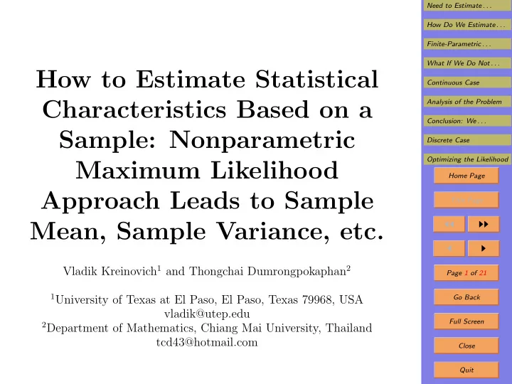
How to Estimate Statistical Continuous Case Characteristics Based - PowerPoint PPT Presentation

Need to Estimate . . . How Do We Estimate . . . Finite-Parametric . . . What If We Do Not . . . How to Estimate Statistical Continuous Case Characteristics Based on a Analysis of the Problem Conclusion: We . . . Sample: Nonparametric Discrete Case Optimizing the Likelihood Maximum Likelihood Home Page Approach Leads to Sample Title Page Mean, Sample Variance, etc. ◭◭ ◮◮ ◭ ◮ Vladik Kreinovich 1 and Thongchai Dumrongpokaphan 2 Page 1 of 21 1 University of Texas at El Paso, El Paso, Texas 79968, USA Go Back vladik@utep.edu Full Screen 2 Department of Mathematics, Chiang Mai University, Thailand tcd43@hotmail.com Close Quit

Need to Estimate . . . How Do We Estimate . . . 1. Need to Estimate Statistical Characteristics Finite-Parametric . . . • In many practical situations, we need to estimate sta- What If We Do Not . . . tistical characteristic based on a given sample. Continuous Case Analysis of the Problem • For example, we need to check that: Conclusion: We . . . – for all the mass-produced gadgets from a given Discrete Case batch, Optimizing the Likelihood – the values of the corresponding physical quantity Home Page are within the desired bounds. Title Page • The ideal solution would be to measure the quantity ◭◭ ◮◮ for all the gadgets. ◭ ◮ • This may be reasonable for a spaceship, where a minor fault can lead to catastrophic results. Page 2 of 21 • Usually, we can save time and money: Go Back – by testing only a small sample, and Full Screen – making statistical conclusions from the results. Close Quit

Need to Estimate . . . How Do We Estimate . . . 2. How Do We Estimate the Statistical Charac- Finite-Parametric . . . teristics – Finite-Parametric Case: Main Idea What If We Do Not . . . • In many situations, we know that the actual distribu- Continuous Case tion belongs to a known finite-parametric family: Analysis of the Problem Conclusion: We . . . f ( x | θ ) for some θ = ( θ 1 , . . . , θ n ) . Discrete Case • For example, the distribution is Gaussian (normal), for Optimizing the Likelihood Home Page some (unknown) mean µ and st. dev. σ . Title Page • In such situations: ◭◭ ◮◮ – we first estimate the values of the parameters θ i based on the sample, and then ◭ ◮ – we compute statistical characteristic (mean, stan- Page 3 of 21 dard deviation, etc.) corr. to the estimates θ i . Go Back Full Screen Close Quit

Need to Estimate . . . How Do We Estimate . . . 3. How Do We Estimate the Statistical Charac- Finite-Parametric . . . teristics – Finite-Parametric Case: Details What If We Do Not . . . • How do we estimate the values of the parameters θ i Continuous Case based on the sample? Analysis of the Problem Conclusion: We . . . • A natural idea is to select the most probable values θ . Discrete Case • How do we go from this idea to an algorithm? Optimizing the Likelihood Home Page • To answer this question, let us first note that: Title Page – while theoretically, each of the parameters θ i can take infinitely many values, ◭◭ ◮◮ – in reality, for a given sample size, ◭ ◮ – it is impossible to detect the difference between the Page 4 of 21 nearby values θ i and θ ′ i . Go Back • Thus, from the practical viewpoint, we have finitely Full Screen many distinguishable cases. Close Quit

Need to Estimate . . . How Do We Estimate . . . 4. Finite-Parametric Case (cont-d) Finite-Parametric . . . • In this description, we have finitely many possible com- What If We Do Not . . . binations of parameters θ (1) , . . . , θ ( N ) . Continuous Case Analysis of the Problem • We consider the case when all we know is that the Conclusion: We . . . actual pdf belongs to the family f ( x | θ ). Discrete Case • There is no a priori reason to consider some of the Optimizing the Likelihood possible values θ ( k ) as more probable. Home Page • Thus, before we start our observations, it is reasonable Title Page to consider these N hypotheses as equally probable: ◭◭ ◮◮ P 0 ( θ ( k ) ) = 1 N . ◭ ◮ Page 5 of 21 • This reasonable idea is known as the Laplace Indeter- Go Back minacy Principle . Full Screen Close Quit

Need to Estimate . . . How Do We Estimate . . . 5. Finite-Parametric Case (cont-d) Finite-Parametric . . . • We can now use the Bayes theorem to compute the What If We Do Not . . . probabilities P ( θ ( k ) | x ) of different hypotheses θ ( k ) Continuous Case Analysis of the Problem – after we have performed the observations, and Conclusion: We . . . – these observations resulted in a sample x = Discrete Case ( x 1 , . . . , x n ): Optimizing the Likelihood P ( x | θ ( k ) ) · P 0 ( θ ( k ) ) Home Page P ( θ ( k ) | x ) = . � N Title Page P ( x | θ ( i ) ) · P 0 ( θ ( i ) ) i =1 ◭◭ ◮◮ • The prob. P ( x | θ ( k ) ) is proportional to f ( x | θ ( k ) ). ◭ ◮ • Dividing both numerator and denominator by P 0 = 1 Page 6 of 21 N , we thus conclude that Go Back P ( θ ( k ) | x ) = c · f ( x | θ ( k ) ) for some constant c. Full Screen Close Quit

Need to Estimate . . . How Do We Estimate . . . 6. Finite-Parametric Case (cont-d) Finite-Parametric . . . • Thus, selecting the most probable hypotheses What If We Do Not . . . P ( θ ( k ) | x ) → max is equivalent to: Continuous Case k Analysis of the Problem – finding the values θ for which, Conclusion: We . . . – for the given sample x , the expression f ( x | θ ) is the Discrete Case largest possible. Optimizing the Likelihood • The expression f ( x | θ ) is known as likelihood . Home Page • The whole idea is thus known as the Maximum Likeli- Title Page hood Method . ◭◭ ◮◮ • In particular, for Gaussian distribution, the Maximum ◭ ◮ Likelihood method leads: Page 7 of 21 � n = 1 def – to the sample mean � µ n · x i , and Go Back i =1 Full Screen n � = 1 σ ) 2 def µ ) 2 . – to the sample variance ( � n · ( x i − � Close i =1 Quit

Need to Estimate . . . How Do We Estimate . . . 7. What If We Do Not Know the Family? Finite-Parametric . . . • Often, we do not know a finite-parametric family of What If We Do Not . . . distributions containing the actual one. Continuous Case Analysis of the Problem • In such situations, all we know is a sample. Conclusion: We . . . • Based on this sample, how can we estimate the statis- Discrete Case tical characteristics of the corresponding distribution? Optimizing the Likelihood Home Page • In this paper, we apply the Maximum Likelihood method to the above problem. Title Page • It turns out that the resulting estimates are sample ◭◭ ◮◮ mean, sample variance, etc. ◭ ◮ • Thus, we get a justification for using these estimates Page 8 of 21 beyond the case of the Gaussian distribution. Go Back Full Screen Close Quit

Need to Estimate . . . How Do We Estimate . . . 8. Continuous Case Finite-Parametric . . . • Let us first consider the case when the random variable What If We Do Not . . . is continuous. Continuous Case Analysis of the Problem • Theoretically, we can thus have infinitely many possi- Conclusion: We . . . ble values of the random variable x . Discrete Case • Ii reality, due to measurement uncertainty, very close Optimizing the Likelihood values x ≈ x ′ are indistinguishable. Home Page • Thus, in practice, we can safely assume that there are Title Page only finitely many distinguishable values ◭◭ ◮◮ x (1) < x (2) < . . . < x ( M ) . ◭ ◮ • To describe the corresponding random variable, we Page 9 of 21 need to describe M probabilities p i = p ( x ( i ) ). Go Back • The only restriction on these probabilities is that they � M Full Screen should be non-negative and add up to 1: p i = 1. Close i =1 Quit

Need to Estimate . . . How Do We Estimate . . . 9. Let Us Apply the Maximum Likelihood Finite-Parametric . . . Method: Resulting Formulation What If We Do Not . . . • According to the Maximum Likelihood Method, Continuous Case Analysis of the Problem – out of all possible probability distributions � p = Conclusion: We . . . ( p 1 , . . . , p n ), Discrete Case – we should select a one for which the probability of Optimizing the Likelihood observing a given sequence x 1 , . . . , x n is the largest. Home Page • The probability of observing each x i is p ( x i ). Title Page • It is usually assumed that different elements in the ◭◭ ◮◮ sample are independent. ◭ ◮ • So, the probability p ( x | � p ) of observing the whole sam- Page 10 of 21 ple x = ( x 1 , . . . , x n ) is equal to the product: Go Back n � p ( x | � p ) = p ( x i ) . Full Screen i =1 Close Quit

Need to Estimate . . . How Do We Estimate . . . 10. Continuous Case (cont-d) Finite-Parametric . . . • In the continuous case, the probability of observing the What If We Do Not . . . exact same number twice is zero. Continuous Case Analysis of the Problem • So, we can safely assume that all the values x i are Conclusion: We . . . different. Discrete Case • In this case, the above product takes the form Optimizing the Likelihood � Home Page p ( x | � p ) = { x i : x i has been observed } . Title Page • We need to find p 1 , . . . , p M that maximize this proba- ◭◭ ◮◮ � M bility under the constraints p i ≥ 0 and p i = 1. ◭ ◮ i =1 Page 11 of 21 Go Back Full Screen Close Quit