Smooth varying coefficient models in Stata Yet another - PowerPoint PPT Presentation
Smooth varying coefficient models in Stata Yet another semiparametric approach Rios-Avila, Fernando 1 1 friosavi@levy.org Levy Economics Institute Stata Conference, July 2020 At home edition Rios-Avila (Levy) vc pack Stata 2020 1 / 38 Table
Smooth varying coefficient models in Stata Yet another semiparametric approach Rios-Avila, Fernando 1 1 friosavi@levy.org Levy Economics Institute Stata Conference, July 2020 At home edition Rios-Avila (Levy) vc pack Stata 2020 1 / 38
Table of Contents Introduction 1 Non-Parametric regressions and SVCM 2 Example 3 SVCM in Stata: vc pack 4 Example: vc pack 5 Conclusions 6 Rios-Avila (Levy) vc pack Stata 2020 2 / 38
Introduction Table of Contents Introduction 1 Non-Parametric regressions and SVCM 2 Example 3 SVCM in Stata: vc pack 4 Example: vc pack 5 Conclusions 6 Rios-Avila (Levy) vc pack Stata 2020 3 / 38
Introduction Introduction Nonparametric regressions are powerful tools to capture relationships between dependent and independent variables with minimal functional forms assumptions. (very flexible) The added flexibility comes at a cost: Curse of dimensionality. Larger sample sizes are needed to achieve same power as parametric models. Computational burden. Procedures for model selection and estimation demand a lot of time. Perhaps because of this, Stata had a limited set of native commands for the estimation of nonparametric models. This changed with npregress series/kernel . (still they kind be slow and too flexible) Rios-Avila (Levy) vc pack Stata 2020 4 / 38
Introduction Introduction A response to the main weakness of NP methods has been the development of semiparametric (SP) methods. SP combine the flexibility of NP regressions with the structure of standard parametric models. The added structure reduces the curse of dimensionality and the computational cost of model selection and estimation. Many community-contributed commands have been proposed for the analysis of a large class of semiparametric models in Stata. See: Verardi(2013) Semipar-Stata Rios-Avila (Levy) vc pack Stata 2020 5 / 38
Introduction Introduction In this presentation, I’ll describe the estimation of a particular type of SP model known as Smooth varying coefficient models (SVCM). Rios-Avila (Levy) vc pack Stata 2020 6 / 38
Introduction Introduction In this presentation, I’ll describe the estimation of a particular type of SP model known as Smooth varying coefficient models (SVCM). I’ll show how they could be estimated ”manually” Rios-Avila (Levy) vc pack Stata 2020 6 / 38
Introduction Introduction In this presentation, I’ll describe the estimation of a particular type of SP model known as Smooth varying coefficient models (SVCM). I’ll show how they could be estimated ”manually” and introduce the package vc pack , that can be used for the model selection, estimation, and visualization of this type of model. Rios-Avila (Levy) vc pack Stata 2020 6 / 38
Non-Parametric regressions and SVCM Table of Contents Introduction 1 Non-Parametric regressions and SVCM 2 Example 3 SVCM in Stata: vc pack 4 Example: vc pack 5 Conclusions 6 Rios-Avila (Levy) vc pack Stata 2020 7 / 38
Non-Parametric regressions and SVCM What do they do? Consider a model with 3 set of variables such that: y = f ( X , Z , e ) Where X and Z are observed and W=[X;Z], E ( e | x , z ) = 0 Rios-Avila (Levy) vc pack Stata 2020 8 / 38
Non-Parametric regressions and SVCM What do they do?:Parametric Regression a Standard OLS (parametric model under linearity assumption), will estimate their relationship with respect to Y such that : E ( y | x , z ) = x ∗ b x + z ∗ b z where its well known that: b w = ( W ′ W ) − 1 ( W ′ Y ) W = [ X ; Z ]& b ′ w = [ b ′ x ; b ′ w ] Rios-Avila (Levy) vc pack Stata 2020 9 / 38
Non-Parametric regressions and SVCM What do they do?:NonParametric Regression NP regression assumes the conditional expected value of the Y is a smooth function. E ( y | x , z ) = g ( x , z ) In this model, often, there are not parameters to be estimated, but conditional means � y i ∗ K ( w i , w , h ) g ( x , z ) = � K ( w i , w , h ) where K () is a product of Kernel functions. (thus this is a kernel-based NP regression) So the NP regression is simply the estimation of weighted means. One can also use Splines, series, or penalized splines. Rios-Avila (Levy) vc pack Stata 2020 10 / 38
Non-Parametric regressions and SVCM What do they do?:SVCM Regression SVCM regression assumes the model is linear conditional on z: E ( y | x , z ) = xb x ( z ) This model combines the linear structure of OLS, assuming the coefficients are nonlinear with respect to Z. If we have enough observations for Z=z, the estimator is simply: b x ( z ) = E ( X ′ X | Z = z ) − 1 E ( X ′ y | Z = z ) b x ( z ) = ( X ′ K ( z ) X ) − 1 ( X ′ K ( z ) y ) where K ( z ) is a matrix with the diagonal equal to the K(Z,z,h). Rios-Avila (Levy) vc pack Stata 2020 11 / 38
Non-Parametric regressions and SVCM What do they do?:SVCM Regression However, local constant tends to be bias at the boundaries of Z. So as an alternative, Local Linear (LL) estimator can be used: b x ( Z i ) ≈ b x ( z ) + ∂ b x ( z ) ( Z i − z ) ∂ z But we are still interested in b x ( z ). The estimator above remains the same, but X is substituted by X = ( X ; ( Z i − z ) X ) Rios-Avila (Levy) vc pack Stata 2020 12 / 38
Example Table of Contents Introduction 1 Non-Parametric regressions and SVCM 2 Example 3 SVCM in Stata: vc pack 4 Example: vc pack 5 Conclusions 6 Rios-Avila (Levy) vc pack Stata 2020 13 / 38
Example SVCM-Kernel Local Linear Estimation The estimation of SVCM is relatively straight forward, specially if Z is a single variable. Choose point(s) of reference Z (probably many points) Choose appropriate bandwidth h Choose between local constant or local linear (or local polynomial) Estimate coefficients, and done Or, use splines instead of kernel (see f able) * Local constant . webuse dui, clear . regress citations college taxes i.csize /// if fines==9 (as if h=0) . regress citations college taxes i.csize /// [iw=normalden(fines,9,.5)] * Local Linear . gen dz=fines-9 . regress citations c.dz##c.(college taxes i.csize) /// [iw=normalden(fines,9,.5)] Rios-Avila (Levy) vc pack Stata 2020 14 / 38
Example Example Rios-Avila (Levy) vc pack Stata 2020 15 / 38
Example Example: Remarks While the estimation is ”easy”, important aspects need to be address: Model selection and choice of bandwidth Systematic model estimation and standard errors. Post estimation and evaluation of the model. and plots of conditional effects. Rios-Avila (Levy) vc pack Stata 2020 16 / 38
SVCM in Stata: vc pack Table of Contents Introduction 1 Non-Parametric regressions and SVCM 2 Example 3 SVCM in Stata: vc pack 4 Example: vc pack 5 Conclusions 6 Rios-Avila (Levy) vc pack Stata 2020 17 / 38
SVCM in Stata: vc pack SVCM in Stata: vc pack To address these points, I propose and present a set of commands that aim to facilitate the estimation of SVMC. In specific, the commands can be used for the estimation of SVCM using a local linear estimator and assuming a single conditioning variable z. Rios-Avila (Levy) vc pack Stata 2020 18 / 38
SVCM in Stata: vc pack Model selection: vc bw and vc bwalt The first (most important) step is the selection of the bandwidth h. This reflects the trade off between variance and Bias in the model estimation. vc bw and vc bwalt provide two options (different algorithms) that can be used to select an optimal bandwidth using a leave-one-out Cross validation procedure: N h ∗ = min h � y − i ) 2 ω ( z )( y i − ˆ i =1 For a faster estimation of the CV criteria and h ∗ , both commands use binned Local Linear regressions. vc_bw[alt] y x1 x2 x3, vcoeff(z) /// [kernel(kfun) trimsample(varname) otheroptions] Rios-Avila (Levy) vc pack Stata 2020 19 / 38
SVCM in Stata: vc pack Binned Regression Rios-Avila (Levy) vc pack Stata 2020 20 / 38
SVCM in Stata: vc pack Estimation and Inference: vc reg; vc bsreg & vc preg The next step is the model estimation. While the estimation itself is simple, the estimation of standard errors require special care. Three options are provided. vc [p|bs]reg These commands estimate LL-SVCM for a selected ”ref. points”. vc [p]reg Estimate VcoV matrix a Sandwich formula: Σ( B ( z )) = q c ( X ′ K ( z ) X ) − 1 ( X ′ K ( z ) D ( e i ) K ( z ) X )( X ′ K ( z ) X ) − 1 The difference between them is how e i is estimated. Either using F-LL or Binn-LL vc bsreg instead uses a Bootstrap procedure to estimate Σ. vc_[p|bs]reg y x1 x2 x3, [vcoeff(z) bw(#) kernel(kfun)] /// [klist(numlist) or k(#) ] /// [robust cluster(varname) hc2 hc3 or reps(#)] Rios-Avila (Levy) vc pack Stata 2020 21 / 38
SVCM in Stata: vc pack Post estimation: vc predict & vc test The third step would be summarize and evaluate the estimated model. This can be done with vc predict & vc test The first command has the following syntax: vc_predict y x1 x2 x3, [ vcoeff(svar) bw(#) kernel(kfun)] /// [yhat(newvar) res(newvar) looe(newvar) lvrg(newvar)] [stest] This command provides some information regarding model fitness. And can be used to obtain model predictions, residuals, Leave-one-out residuals, or the leverage statistics option stest , estimates the approximate F-Statistic for testing against parametric models. Rios-Avila (Levy) vc pack Stata 2020 22 / 38
Recommend
More recommend
Explore More Topics
Stay informed with curated content and fresh updates.
