How black-box use of imputation can cause bias Nicole Erler Erasmus - PowerPoint PPT Presentation
How black-box use of imputation can cause bias Nicole Erler Erasmus Medical Center, Rotterdam Nicole Erler, FGME 2019, Kiel 1 Handling Missing Values is Easy! Functions automatically exclude missing values: ## [...] ## Residual standard
How black-box use of imputation can cause bias Nicole Erler Erasmus Medical Center, Rotterdam Nicole Erler, FGME 2019, Kiel 1
Handling Missing Values is Easy! Functions automatically exclude missing values: ## [...] ## Residual standard error: 2.305 on 69 degrees of freedom ## (25 observations deleted due to missingness) ## Multiple R-squared: 0.09255, Adjusted R-squared: 0.02679 ## F-statistic: 1.407 on 5 and 69 DF, p-value: 0.2325 Nicole Erler, FGME 2019, Kiel 2
Handling Missing Values is Easy! Functions automatically exclude missing values: ## [...] ## Residual standard error: 2.305 on 69 degrees of freedom ## (25 observations deleted due to missingness) ## Multiple R-squared: 0.09255, Adjusted R-squared: 0.02679 ## F-statistic: 1.407 on 5 and 69 DF, p-value: 0.2325 Imputation is super easy: library ("mice") imp <- mice (mydata) However ... Nicole Erler, FGME 2019, Kiel 2
Handling Missing Values Correctly is Not So Easy! (Imputation) methods makes certain assumptions , e.g.: missingness is M(C)AR Nicole Erler, FGME 2019, Kiel 3
Handling Missing Values Correctly is Not So Easy! (Imputation) methods makes certain assumptions , e.g.: missingness is M(C)AR the incomplete variable has a certain conditional distribution (e.g. normal) Nicole Erler, FGME 2019, Kiel 3
Handling Missing Values Correctly is Not So Easy! (Imputation) methods makes certain assumptions , e.g.: missingness is M(C)AR the incomplete variable has a certain conditional distribution (e.g. normal) all associations are linear no interactions no non-linear effects no transformations Nicole Erler, FGME 2019, Kiel 3
Handling Missing Values Correctly is Not So Easy! (Imputation) methods makes certain assumptions , e.g.: missingness is M(C)AR the incomplete variable has a certain conditional distribution (e.g. normal) all associations are linear no interactions no non-linear effects no transformations compatibility of the imputation models congeniality (compatibility between analysis and imputation models) Nicole Erler, FGME 2019, Kiel 3
Handling Missing Values Correctly is Not So Easy! (Imputation) methods makes certain assumptions , e.g.: missingness is M(C)AR the incomplete variable has a certain conditional distribution (e.g. normal) all associations are linear no interactions no non-linear effects no transformations compatibility of the imputation models congeniality (compatibility between analysis and imputation models) violation ➡ bias Nicole Erler, FGME 2019, Kiel 3
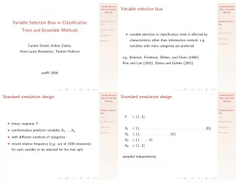
Literature: mis-specification in Multiple Imputation Several authors have investigated robustness to mis-specification (of distribution) in MI using FCS / MICE in joint model MI and/or proposed to use Tukey’s gh distribution Fleishman polynomials GAMs (in FCS) Doubly-robust weighted estimating equations (instead of MI) Nicole Erler, FGME 2019, Kiel 4
Fully Bayesian Analysis & Imputation Joint distribution p ( y | X , b , θ ) p ( X | θ ) p ( b | θ ) p ( θ ) � �� � � �� � � �� � ���� imputation priors analysis random model part effects Nicole Erler, FGME 2019, Kiel 5
Fully Bayesian Analysis & Imputation Joint distribution p ( y | X , b , θ ) p ( X | θ ) p ( b | θ ) p ( θ ) � �� � � �� � � �� � ���� imputation priors analysis random model part effects Imputation part X � �� � p ( x 1 , . . . , x p , X compl . | θ ) = p ( x 1 | X compl . , θ ) p ( x 2 | X compl . , x 1 , θ ) p ( x 3 | X compl . , x 1 , x 2 , θ ) . . . Nicole Erler, FGME 2019, Kiel 5
Fully Bayesian Analysis & Imputation Joint distribution p ( y | X , b , θ ) p ( X | θ ) p ( b | θ ) p ( θ ) � �� � � �� � � �� � ���� imputation priors analysis random model part effects Imputation part X � �� � p ( x 1 , . . . , x p , X compl . | θ ) = p ( x 1 | X compl . , θ ) p ( x 2 | X compl . , x 1 , θ ) p ( x 3 | X compl . , x 1 , x 2 , θ ) . . . Software Implemented in the R package JointAI Nicole Erler, FGME 2019, Kiel 5
MICE vs JointAI Imputation in MICE Imputation in JointAI p ( y | X compl . , x 1 , x 2 , x 3 , . . . , θ ) p ( x 1 | y , X compl . , x 2 , x 3 , x 4 , . . . , θ ) p ( x 1 | X compl . , θ ) p ( x 2 | y , X compl . , x 1 , x 3 , x 4 , . . . , θ ) p ( x 2 | X compl . , x 1 , θ ) p ( x 3 | y , X compl . , x 1 , x 2 , x 4 , . . . , θ ) p ( x 3 | X compl . , x 1 , x 2 , θ ) . . . . . . Nicole Erler, FGME 2019, Kiel 6
MICE vs JointAI Imputation in MICE Imputation in JointAI p ( y | X compl . , x 1 , x 2 , x 3 , . . . , θ ) p ( x 1 | y , X compl . , x 2 , x 3 , x 4 , . . . , θ ) p ( x 1 | X compl . , θ ) p ( x 2 | y , X compl . , x 1 , x 3 , x 4 , . . . , θ ) p ( x 2 | X compl . , x 1 , θ ) p ( x 3 | y , X compl . , x 1 , x 2 , x 4 , . . . , θ ) p ( x 3 | X compl . , x 1 , x 2 , θ ) . . . . . . No issues with complex outcomes, e.g.: multi-level survival congeniality compatibility Nicole Erler, FGME 2019, Kiel 6
MICE vs JointAI Imputation in MICE Imputation in JointAI p ( y | X compl . , x 1 , x 2 , x 3 , . . . , θ ) p ( x 1 | y , X compl . , x 2 , x 3 , x 4 , . . . , θ ) p ( x 1 | X compl . , θ ) p ( x 2 | y , X compl . , x 1 , x 3 , x 4 , . . . , θ ) p ( x 2 | X compl . , x 1 , θ ) p ( x 3 | y , X compl . , x 1 , x 2 , x 4 , . . . , θ ) p ( x 3 | X compl . , x 1 , x 2 , θ ) . . . . . . ➡ ➡ Potential mis-specification of association structure conditional distribution M(C)AR Nicole Erler, FGME 2019, Kiel 7
Simulation Study: Quadratic Effect Analysis model: y ∼ β 0 + β 1 x 1 + β 2 x 2 + . . . Quadratic association between covariates: x 1 ∼ α 0 + α 1 x 2 + ❍❍ α 2 x 2 2 + . . . ❍ x 1 (incomplete covariate) 30 20 10 0 −10 −2 0 2 −2 0 2 −2 0 2 x 2 (complete covariate) Nicole Erler, FGME 2019, Kiel 8
Simulation Study: Quadratic Effect Analysis model: y ∼ β 0 + β 1 x 1 + β 2 x 2 + . . . Quadratic association between covariates: x 1 ∼ α 0 + α 1 x 2 + ❍❍ α 2 x 2 2 + . . . ❍ x 1 (incomplete covariate) 30 20 10 0 −10 −2 0 2 −2 0 2 −2 0 2 x 2 (complete covariate) 2.0 10% NA 1.8 30% NA 1.6 relative bias 50% NA 1.4 1.2 1.0 0.8 0.6 mice JointAI mice JointAI mice JointAI Nicole Erler, FGME 2019, Kiel 8
Simulation Study: Logarithmic Effect Analysis model: y ∼ β 0 + β 1 x 1 + β 2 x 2 + . . . Log-association between covariates: x 1 ∼ α 0 + α 1 ❩ log( x 2 ) + . . . ❩ x 1 (incomplete covariate) 4 0 −4 −8 −12 0.4 0.8 1.2 0.4 0.8 1.2 0.4 0.8 1.2 x 2 (complete covariate) 1.8 1.6 1.4 relative bias 1.2 1.0 0.8 0.6 10% NA 0.4 30% NA 0.2 50% NA mice JointAI mice JointAI mice JointAI Nicole Erler, FGME 2019, Kiel 9
Simulation Study: Gamma distribution Analysis model: y ∼ β 0 + β 1 x 1 + β 2 x 2 + . . . Gamma-distributed covariate: x 1 | x 2 , x 3 , . . . ∼ Ga () conditional distribution 2.0 1.5 1.0 0.5 0.0 0 2 4 6 0 2 4 6 0 2 4 6 x 1 (incomplete covariate) 2.0 10% NA 1.8 30% NA relative bias 1.6 50% NA 1.4 1.2 1.0 0.8 mice JointAI mice JointAI mice JointAI Nicole Erler, FGME 2019, Kiel 10
Flexible Bayesian Models We need more flexible imputation models! Ideally: models that fit (almost) any distribution / association structure. Nicole Erler, FGME 2019, Kiel 11
Flexible Bayesian Models We need more flexible imputation models! Ideally: models that fit (almost) any distribution / association structure. Ideas: flexible association structure: penalized splines flexible residual distribution : mixture of Polya-Trees Nicole Erler, FGME 2019, Kiel 11
Bayesian P-Splines d � Instead of β 1 x 2 we use β ℓ B ℓ ( x 2 ): ℓ =1 ● ● ● ● ● ● ● ● ● ● ●● ● ● ● ● ● ● ● ● ● ● ● ● ● ● ● ● ● ● ● ● ● ● ● ● ● ● ● ● ● ● ● ● ● ● ● ● ● ● ● ● ● ● ● ● ● ● ● ● ● ● ● ● ● ● ● ● ● ● ● ● ● ● ● ● ● ● ● ● ● ● ● ● ● ● ● ● ● ● ● ● ● ● ● ● ● ● ● ● ● ● ● ● ● ● ● ● ● ● ● ● ● ● ● ● ● ● ● ● ● ● ● ● ● ● ● ● ● ● ● ● ● ● ●● ● ● ● ● ● ● ● ● ● ● ● ● ● ● ● ● ● ● ● ● ● ● ● ● ● ● ● ● x 1 ● ● ● ● ● ● ● ● ● ● ● ● ● ● ●● ● ● ● ● ● ● ● ● ● ● ● ● ●● ● ● ● ● ● ● ● ● ● ● ● ● ● ● ● ● ● ● ● ● ● ● ● ● ● ● ● ● ● ● ● ● ● ● ● ● ● ● ● ● ● ● ● ● ● ● ● ● ● ● ● ● ● ● ● ● x 2 Nicole Erler, FGME 2019, Kiel 12
Recommend
More recommend
Explore More Topics
Stay informed with curated content and fresh updates.







![[7] Gaussian Elimination Starting to peek inside the black box So far sol ve( A, b) is a black](https://c.sambuz.com/898910/7-gaussian-elimination-starting-to-peek-inside-the-black-s.webp)


