Gaussian Elimination [7] Gaussian Elimination
Starting to peek inside the black box So far sol ve( A, b) is a black box. With Gaussian elimination, we begin to find out what’s inside.
Starting to peek inside the black box So far sol ve( A, b) is a black box. With Gaussian elimination, we begin to find out what’s inside.
Gaussian Elimination: Origins Method illustrated in Chapter Eight of a Chinese text, The Nine Chapters on the Mathematical Art , that was written roughly two thousand years ago. Rediscovered in Europe by Isaac Newton (England) and Michel Rolle (France) Gauss called the method eliminiationem vulgarem (“common elimination”) Gauss adapted the method for another problem (one we study soon) and developed notation.
Gaussian elimination: Uses I Finding a basis for the span of given vectors . This additionally gives us an algorithm for rank and therefore for testing linear dependence. I Solving a matrix equation ,which is the same as expressing a given vector as a linear combination of other given vectors , which is the same as solving a system of linear equations I Finding a basis for the null space of a matrix , which is the same as finding a basis for the solution set of a homogeneous linear system , which is also relevant to representing the solution set of a general linear system.
Echelon form Echelon form a generalization of triangular matrices 2 3 0 2 3 0 5 6 0 0 1 0 3 4 6 7 Example: 6 7 0 0 0 0 1 2 4 5 0 0 0 0 0 9 Note that I the first nonzero entry in row 0 is in column 1, I the first nonzero entry in row 1 is in column 2, I the first nonzero entry in row 2 is in column 4, and I the first nonzero entry in row 4 is in column 5. Definition: An m × n matrix A is in echelon form if it satisfies the following condition: for any row, if that row’s first nonzero entry is in position k then every previous row’s first nonzero entry is in some position less than k .
Echelon form Definition: An m × n matrix A is in echelon form if it satisfies the following condition: for any row, if that row’s first nonzero entry is in position k then every previous row’s first nonzero entry is in some position less than k . This definition implies that, as you iterate through the rows of A , the first nonzero entries per row move strictly right, forming a sort of staircase that descends to the right. 2 1 0 4 1 3 9 7 0 6 0 1 3 0 4 1 0 0 0 0 2 1 3 2 2 3 2 3 0 2 3 0 5 6 4 1 3 0 0 0 0 0 0 0 0 1 0 0 1 0 3 4 0 3 0 1 6 7 6 7 6 7 6 7 0 0 0 0 1 2 0 0 1 7 4 5 4 5 0 0 0 0 0 9 0 0 0 9
Echelon form Definition: An m × n matrix A is in echelon form if it satisfies the following condition: for any row, if that row’s first nonzero entry is in position k then any previous row’s first nonzero entry is in some position less than k . If a row of a matrix in echelon form is all zero then every subsequent row must also be all zero, e.g. 2 3 0 2 3 0 5 6 0 0 1 0 3 4 6 7 6 7 0 0 0 0 0 0 4 5 0 0 0 0 0 0
Uses of echelon form What good is it having a matrix in echeleon form? Lemma: If a matrix is in echelon form, the nonzero rows form a basis for the row space. For example, a basis for the row space of 2 3 0 2 3 0 5 6 0 0 1 0 3 4 6 7 6 7 0 0 0 0 0 0 4 5 0 0 0 0 0 0 is { [0 , 2 , 3 , 0 , 5 , 6] , [0 , 1 , 0 , 3 , 4] } . In particular, if every row is nonzero, as in each of the matrices 2 3 2 3 2 3 0 2 3 0 5 6 2 1 0 4 1 3 9 7 4 1 3 0 0 0 1 0 3 4 0 6 0 1 3 0 4 1 0 3 0 1 6 7 6 7 6 7 5 , 5 , 6 7 6 7 6 7 0 0 0 0 1 2 0 0 0 0 2 1 3 2 0 0 1 7 4 4 4 5 0 0 0 0 0 9 0 0 0 0 0 0 0 1 0 0 0 9 then the rows form a basis of the row space.
Uses of echelon form Lemma: If matrix is in echelon form, the nonzero rows form a basis for row space. It is obvious that the nonzero rows span the row space. We need only show that these vectors are linearly independent. We prove it using the Grow algorithm: 2 3 def Grow ( V ) 4 1 3 0 S = ∅ 0 3 0 1 6 7 6 7 repeat while possible: 0 0 1 7 4 5 find a vector v in V that is not in Span S , and put it in S 0 0 0 9 We run the Grow algorithm, adding rows of matrix in reverse order to S : I Since Span ∅ does not include [0 , 0 , 0 , 9], the algorithm adds this vector to S . I Now S = { [0 , 0 , 0 , 9] } . Every vector in Span S has zeroes in positions 0, 1, 2, so Span S does not contain [0 , 0 , 1 , 7], so the algorithm adds this vector to S . I Now S = { [0 , 0 , 0 , 9] , [0 , 0 , 1 , 7] } . Every vector in Span S has zeroes in positions 0, 1, so Span S does not contain [0 , 3 , 0 , 1], so the algorithm adds it. I Now S = { [0 , 0 , 0 , 9] , [0 , 0 , 1 , 7] , [0 , 3 , 0 , 1] } . Every vector in Span S has a zero in position 0, so Span S does not contain [4 , 1 , 3 , 0], so the algorithm adds it, and we are done.
Transforming a matrix to echelon form Lemma: If matrix is in echelon form, the nonzero rows form a basis for row space. Suggests an approach: To find basis for row space of a matrix A , iteratively transform A into a matrix B I in echelon form I with no zero rows I whose row space is the same as that of A . We will represent current matrix as a rowlist. Assume r ow l i st has been initialized with a list of Vecs, e.g.. A � B C A B C A B C r ow l i st = 2 , 3 , 0 1 1 2 0 0 1 We will mutate this variable. To handle Vecs with arbitrary D , must decide on an ordering: col _l abel _l i st = sor t ed( r ow l i st [ 0] . D , key=st r )
First attempt: Sorting rows by position of the leftmost nonzero Goal: Transform a matrix r ow l i st into a matrix new r ow l i st in echelon form. Here’s an easy matrix to start with: A B C D E F A B C D E F 0 0 2 3 0 5 6 0 0 0 0 0 1 2 1 0 2 3 0 5 6 2 0 0 0 0 0 0 3 0 0 1 0 3 4 Suggests an algorithm: sort the rows according to position of leftmost nonzero entry.
First attempt: Sorting rows by position of the leftmost nonzero Goal: Transform a matrix r ow l i st into a matrix new r ow l i st in echelon form. Here’s an easy matrix to start with: A B C D E F A B C D E F 0 0 2 3 0 5 6 0 0 0 0 0 1 2 1 0 0 1 0 3 4 1 0 2 3 0 5 6 2 0 0 0 0 0 0 3 0 0 1 0 3 4 Suggests an algorithm: sort the rows according to position of leftmost nonzero entry.
First attempt: Sorting rows by position of the leftmost nonzero Goal: Transform a matrix r ow l i st into a matrix new r ow l i st in echelon form. Here’s an easy matrix to start with: A B C D E F A B C D E F 0 0 2 3 0 5 6 0 0 0 0 0 1 2 1 0 0 1 0 3 4 1 0 2 3 0 5 6 2 0 0 0 0 1 2 2 0 0 0 0 0 0 3 0 0 1 0 3 4 Suggests an algorithm: sort the rows according to position of leftmost nonzero entry.
First attempt: Sorting rows by position of the leftmost nonzero Goal: Transform a matrix r ow l i st into a matrix new r ow l i st in echelon form. Here’s an easy matrix to start with: A B C D E F A B C D E F 0 0 2 3 0 5 6 0 0 0 0 0 1 2 1 0 0 1 0 3 4 1 0 2 3 0 5 6 2 0 0 0 0 1 2 2 0 0 0 0 0 0 3 0 0 0 0 0 0 3 0 0 1 0 3 4 Suggests an algorithm: sort the rows according to position of leftmost nonzero entry.
Sorting rows by position of the leftmost nonzero Goal: a method of transforming a rowlist into one that is in echelon form. First attempt: Sort the rows by position of the leftmost nonzero entry. We will use a naive algorithm of sorting: I first choose a row with a nonzero in first column, I then choose a row with a nonzero in second column, . . . accumulating these in a list new r ow l i st , initially empty: new _r ow l i st = [ ] The algorithm maintains the set of indices of rows remaining to be sorted, r ow s l ef t , initially consisting of all the row indices: r ow s_l ef t = set ( r ange( l en( r ow l i st ) ) )
Sorting rows by position of the leftmost nonzero col _l abel _l i st = sor t ed( r ow l i st [ 0] . D , key=st r ) new _r ow l i st = [ ] r ow s_l ef t = set ( r ange( l en( r ow l i st ) ) ) I Algorithm iterates through the column labels in order. I In each iteration, algorithm finds a list r ow s w i t h nonzer o of indices of the remaining rows that have nonzero entries in the current column I Algorithm selects one of these rows (the pivot row ), adds it to new r ow l i st , and removes its index from r ow s l ef t . f or c i n col _l abel _l i st : r ow s_w i t h_nonzer o = [ r f or r i n r ow s_l ef t i f r ow l i st [ r ] [ c] ! = 0] pi vot = r ow s_w i t h_nonzer o[ 0] new _r ow l i st . append( r ow l i st [ pi vot ] ) r ow s_l ef t . r em ove( pi vot )
Recommend
More recommend
Unleash a World of Digital Possibilities—Browse, Share, and Explore Content Without Boundaries
![[8] The Inner Product Continuing to look inside the black box We studied Gaussian elimination,](https://c.sambuz.com/784282/8-the-inner-product-continuing-to-look-inside-the-black-s.webp)