Chapter 9: Gaussian Elimination ES 240: Scientific and Engineering - PowerPoint PPT Presentation
ES 240: Scientific and Engineering Computation. Chapter 9: Gaussian Elimination Uchechukwu Ofoegbu Temple University Chapter 9: Gaussian Elimination ES 240: Scientific and Engineering Computation. Chapter 9: Gaussian Elimination Graphical
ES 240: Scientific and Engineering Computation. Chapter 9: Gaussian Elimination Uchechukwu Ofoegbu Temple University Chapter 9: Gaussian Elimination
ES 240: Scientific and Engineering Computation. Chapter 9: Gaussian Elimination Graphical Method Graphical Method � The solution of a small set of simultaneous equations, can be obtained by graphing them and determining the location of the intercept
ES 240: Scientific and Engineering Computation. Chapter 9: Gaussian Elimination Graphical Method (cont) Graphical Method (cont) � Graphing the equations can also show systems where: a) No solution exists – The coefficient matrix is singular (determinant = 0) b) Infinite solutions exist – The coefficient matrix is singular (determinant = 0) c) System is ill-conditioned – The coefficient matrix is almost singular (determinant ≈ 0)
ES 240: Scientific and Engineering Computation. Chapter 9: Gaussian Elimination Determinants Determinants � The determinant D =| A | of a matrix is formed from the coefficients of [A]. � Determinants for small matrices are: 1 × 1 a 11 = a 11 a 11 a 12 2 × 2 = a 11 a 22 − a 12 a 21 a 21 a 22 a 11 a 12 a 13 a 22 a 23 a 21 a 23 a 21 a 22 3 × 3 = a 11 − a 12 + a 13 a 21 a 22 a 23 a 32 a 33 a 31 a 33 a 31 a 32 a 31 a 32 a 33 � Determinants for matrices larger than 3 x 3 can be very complicated.
ES 240: Scientific and Engineering Computation. Chapter 9: Gaussian Elimination Example Example � Find the determinants of the following matrices: 0 . 5 1 . 9 = A 0 . 1 0 . 5 0 . 3 0 . 52 1 = B 0 . 5 1 1 . 9 0 . 1 0 . 3 0 . 5
ES 240: Scientific and Engineering Computation. Chapter 9: Gaussian Elimination Cramer’ ’s Rule s Rule Cramer � Definition: – each unknown in a system of linear algebraic equations may be expressed as a fraction of two determinants with denominator D and with the numerator obtained from D by replacing the column of coefficients of the unknown in question by the constants b 1 , b 2 , …, b n .
ES 240: Scientific and Engineering Computation. Chapter 9: Gaussian Elimination Cramer’ ’s Rule Example s Rule Example Cramer � Find x 2 in the following system of equations: 0.3 x 1 + 0.52 x 2 + x 3 = − 0.01 0.5 x 1 + x 2 + 1.9 x 3 = 0.67 0.1 x 1 + 0.3 x 2 + 0.5 x 3 = − 0.44 � Find the determinant D of the coefficient matrix 0 . 3 0 . 52 1 1 1 . 9 0 . 5 1 . 9 0 . 5 1 = = − + = − D 0 . 5 1 1 . 9 0 . 3 0 . 52 1 0 . 0022 0 . 3 0 . 5 0 . 1 0 . 5 0 . 1 0 . 4 0 . 1 0 . 3 0 . 5 � Find determinant D 2 by replacing D ’s second column with b − 0.01 0.3 1 = 0.3 0.67 1.9 0.5 − 0.010.5 1.9 0.5 + 10.5 0.67 D 2 = − 0.44 = 0.0649 0.5 0.67 1.9 − 0.44 0.1 0.1 − 0.44 0.1 0.5 � Divide x 2 = D 2 D = 0.0649 − 0.0022 = − 29.5
ES 240: Scientific and Engineering Computation. Chapter 9: Gaussian Elimination Naï ïve Gauss Elimination ve Gauss Elimination Na � For larger systems, Cramer’s Rule can become unwieldy. � Instead, a sequential process of removing unknowns from equations using forward elimination followed by back substitution may be used - this is Gauss elimination. � “Naïve” Gauss elimination simply means the process does not check for potential problems resulting from division by zero.
ES 240: Scientific and Engineering Computation. Chapter 9: Gaussian Elimination Naï ïve Gauss Elimination (cont) ve Gauss Elimination (cont) Na � Forward elimination – Starting with the first row, add or subtract multiples of that row to eliminate the first coefficient from the second row and beyond. – Continue this process with the second row to remove the second coefficient from the third row and beyond. – Stop when an upper triangular matrix remains. � Back substitution – Starting with the last row, solve for the unknown, then substitute that value into the next highest row. – Because of the upper-triangular nature of the matrix, each row will contain only one more unknown.
ES 240: Scientific and Engineering Computation. Chapter 9: Gaussian Elimination Gauss Program Efficiency Gauss Program Efficiency � The execution of Gauss elimination depends on the amount of floating-point operations (or flops). The flop count for an n x n system is: 2 n 3 ( ) Forward 3 + O n 2 Elimination n 2 + O n Back ( ) Substitution 2 n 3 ( ) 3 + O n 2 Total � Conclusions: – As the system gets larger, the computation time increases greatly. – Most of the effort is incurred in the elimination step.
ES 240: Scientific and Engineering Computation. Chapter 9: Gaussian Elimination Pivoting Pivoting � Problems arise with naïve Gauss elimination if a coefficient along the diagonal is 0 (problem: division by 0) or close to 0 (problem: round-off error) � One way to combat these issues is to determine the coefficient with the largest absolute value in the column below the pivot element. The rows can then be switched so that the largest element is the pivot element. This is called partial pivoting. � If the rows to the right of the pivot element are also checked and columns switched, this is called complete pivoting .
ES 240: Scientific and Engineering Computation. Chapter 9: Gaussian Elimination Example Example Using the Gaussian Elimination method, solve: − + = ⎧ ⎫ 2 3 1 2 x y z ⎪ ⎪ − + − = − ⎨ ⎬ 4 x y 2 z 1 ⎪ ⎪ − + + = − ⎩ ⎭ 1 x 2 y 3 z 9
ES 240: Scientific and Engineering Computation. Chapter 9: Gaussian Elimination Example Example � Open the GaussPivot function � Use the Gauss Pivot function to solve the problem instead
ES 240: Scientific and Engineering Computation. Chapter 9: Gaussian Elimination Lab Lab � Ex 9.6 – by hand – Using matlab colon operations – Using the GaussPivot function
Recommend
More recommend
Explore More Topics
Stay informed with curated content and fresh updates.
![[7] Gaussian Elimination Starting to peek inside the black box So far sol ve( A, b) is a black](https://c.sambuz.com/898910/7-gaussian-elimination-starting-to-peek-inside-the-black-s.webp)
