HAUSDORFF DIMENSIONS FOR RANDOM WALKS AND THEIR WINDING SECTORS - PowerPoint PPT Presentation
HAUSDORFF DIMENSIONS FOR RANDOM WALKS AND THEIR WINDING SECTORS LPTMS ORSAY CNRS/Universit e Paris-Sud with Jean Desbois JSTAT (2008) P08004 arXiv: 0804.1002 about some recent numerical simulations for random walks on a square lattice
HAUSDORFF DIMENSIONS FOR RANDOM WALKS AND THEIR WINDING SECTORS LPTMS ORSAY CNRS/Universit´ e Paris-Sud with Jean Desbois JSTAT (2008) P08004 arXiv: 0804.1002 about some recent numerical simulations for random walks on a square lattice → Brownian curves in the continuous limit (in particular their Hausdorff dimensions) new definition of a Brownian frontier → new Hausdorff dimension ?
as it is well known: the Hausdorff dimension of the external frontier of Brownian curves is d H = 4 / 3 (numerical conjecture by Mandelbrot, proved by SLE: Lawler, Schramm, Werner ”The dimension of the planar Brownian frontier is 4 / 3” Mathematical Research Letters 8 (2001)) Hausdorff dimension d H P = perimeter of the frontier and r = typical size scaling P = r d H -for example for a circle P = 2 π r ⇒ d H = 1 -for Brownian curves: the external frontier is defined ”geometrically” as the set of points where one stops when one meets the curve for the first time arriving from infinity → no excursion inside the curve and problem of orientation for the frontier
the question asked: can we define the frontier in a different way → oriented Some ideas from: - site percolation on a square lattice - recent progress on Brownian winding sectors (SLE) → 0-winding sectors ⇒ excursions inside the curve
site percolation on a square lattice: probability 0 < p < 1 on each site of a square lattice draw randomly a number 0 < α < 1: if α > p → insulator (white) if α < p → conductor (black) percolation means: -current flows if at least one edge in common -current does not flow if one vertex in common critical percolation: at p c = 0 . 593 ... (numerical) the percolating cluster scales like the overall size of the lattice still there are non percolating sectors inside the cluster: -fjords = non percolating sectors which can be connected to the exterior (since the current does not flow) -lakes = non percolating sectors which cannot be connected to the exterior (deep inside the cluster)
An example: b) a) c) a) site percolation cluster b) external frontier c) external + fjords frontier
Hausdorff dimension: scaling of the perimeter P with the typical size r of the cluster at critical percolation r ≃ size of the lattice -for the perimeter of the external frontier of the cluster: d H = 4 / 3 -for the perimeter of the external +fjords frontier: d H = 7 / 4 external 4 / 3 → excursion around the fjords 7 / 4 Can something analogous to fjords and lakes can be defined for Brownian curves ?
2d Brownian curves: random walk on a square lattice a : probability 1 / 4 → up, down, left, right number of steps N ⇒ continuum limit N → ∞ , a → 0 with Na 2 = 2 t fixed t is the time ⇒ infinite length Na → ∞ r at time → in the continuum: probability for the Brownian particle to reach � t starting from � r 0 at time 0 r − r 0 ) 2 / 2 t G ( r , t / r 0 , 0 ) = 2 π t e − ( 1 � � � � i.e. free 2d quantum propagator � d 2 � r 0 ) 2 > = r 0 ) 2 = 2 t r − � rG ( r , t / r 0 , 0 )( r − � ⇒ < ( � � � � √ → typical size of a Brownian curve after time t : r = 2 t regularized length : a ( Na ) = 2 t = r 2 ⇒ surface filling curve d H = 2 (circle) perimeter of the external frontier : P = r 4 / 3 ⇒ d H = 4 / 3
Look inside the curve: n -winding sectors= connected set of points enclosed n times by the curve a) b) 0 0 1 1 1 1 2 2 1 1 0 0 1 1 B A 0 0 C 0 0 0 0 −1 −1 −1 −1 −2 −2 1 1 0 0 −1 −1 0 c) 1 1 2 1 0 1 0 0 0 −1 −1 −2 1 0 −1 a) a closed Brownian curve with winding sectors n = − 2 , − 1 , 0 , 1 , 2
Comtet, Desbois, S.O. (1990) random variable S n = arithmetic area of the n -winding sectors inside a Brownian curve of length t scaling properties of Brownian curves → S n scales like t average < S n > on all closed curves of length t can be computed by path integral technics
� t r 2 ( τ ) ˙ r ( t )= r � r 0 ) 2 / 2 t = � � � d τ r − path integral: G ( r , t / r 0 , 0 ) = 2 π t e − ( r 0 D re − 1 � � � � � 0 2 r ( 0 )= � � r ( t ) = � r 0 closed curve � probability P ( r 0 , n , t ) to wind n times around the origin after time t : � � t θ = 2 π n → n = 1 θ d τ 0 ˙ 2 π � t � 1 0 e i 2 πα ( n − 1 θ d τ ) d α 0 ˙ ⇒ constraint δ n , 1 � t θ d τ = 2 π 0 ˙ 2 π � t r 2 ( τ ) ˙ � 1 r ( t )= r 0 � 0 d α e i 2 πα n � � + i α ˙ θ ) d τ � in the path integral P ( r 0 , n , t ) = r 0 D re − 0 ( � � 2 r ( 0 )= � � � in the action α ˙ θ = � A vector potential = α ∂θ ⇒ quantum particle A . ˙ r → � � coupled to an Aharanov-Bohm flux 2 πα at the origin set of all closed curves of length t : integrate over � r 0 � d � � 1 0 d α e i 2 πα n Z t ( α ) → P ( n , t ) = r 0 P ( r 0 , n , t ) = � Z t ( α ) = Aharonov-Bohm partition function (with β → t ) S n = arithmetic area n -winding sectors → B field also needed ⇒ the result :
t n � = 0 : < S n > = 2 π n 2 n = 0 : < S 0 > = ∞ since outside 0-winding sea necessarily included r 0 ) (integration over initial point � ⇒ < S 0 > inside the curve not known 1994: W. Werner thesis : ”Sur l’ensemble des points autour desquels le mouvement Brownien plan tourne beaucoup” t when n → ∞ one has n 2 S n → < n 2 S n > = 2 π 2005: Garban, Trujillo Ferreras ”The expected area of the filled planar Brownian loop is π / 5” SLE → total arithmetic area known < S > = t π 5 = < S 0 > + 2 ∑ ∞ n = 1 < S n > ⇒ < S 0 > = t π 30 → pay more attention to the 0-winding sectors which can be connected to the outside (like percolation fjords)
a simple example a) b) 0 0 −1 −1 0 0 +1 +1 0 0 0 0 c) 0 0 −1 +1 +1 −1 0 0 a) closed random walk and winding sectors b) same walk with an oriented frontier (the fjord is opened)
a) and b) are two possible time histories of the same random path ⇒ always possible to follow a time history such that one can define a frontier - on one side 0-winding sector and on the other side ± 1-winding sector -different from usual exterior (geometric) non oriented frontier -excursions inside the walk around the fjords → oriented frontier = external + fjords frontier
a) b) 0 0 1 1 1 1 2 2 1 1 0 0 1 1 B A 0 0 C 0 0 0 0 −1 −1 −1 −1 −2 −2 1 1 0 0 −1 −1 0 c) 1 1 2 1 0 1 0 0 0 −1 −1 −2 1 0 −1 ⇒ 0-windings=fjords + lakes: remain inside the curve (as in percolation)
in red a closed random walk N = 1000000 in blue the fjords, in green the lakes: the fjords remain on the boundary of the walk; the lakes proliferate inside the walk.
numerical simulation for random walks on a square lattice ( N : 10 4 → 10 7 ) 1e+06 c) b) 100000 a) 10000 1000 100 1000 <r > a)external (geometric) frontier g b)external+fjords (oriented) frontier c)external+fjords+lakes(disconnected) : the slopes are a) and b)= 4/3 and c) = 1 . 77 ≈ 7 / 4
numerics: -small N ≃ 10000 → big statistics needed → up to 100000 curves -big N ≃ 10000000 → up to 30000 curves for a given N : -for each curve estimate P and r -deduce < P > and < r > ⇒ a point in the plot
- Hausdorff dimension of the perimeter of the external+fjords oriented frontier d H = 4 3 same as the external frontier → the fjords are subleading in the continuum take also into account the lakes ⇒ disconnected frontier: - Hausdorff dimension of the perimeter of the external+fjords+lakes frontier d H = 7 4 ⇒ 4 / 3 → 7 / 4 due to the lakes proliferation : leading in the continuum
if you take the same point of view in percolation: (numerical simulation with lattice size up to 3200 × 3200) - Hausdorff dimension of the perimeter of the external+fjords+lakes disconnected frontier d H ≃ 1 . 9 → 91 48 Summary BROWNIAN PERCOLATION exterior 4 exterior 4 3 3 exterior+fjords 4 exterior+fjords 7 3 4 exterior+fjords+lakes 7 exterior+fjords+lakes 91 4 48 91 / 48: same dimension as the mass (i.e. area) of the percolating cluster
percolation: mass of the object (i.e. area) ≃ perimeter : d H = 91 48 very porous Brownian: the same thing happens < S > = π t / 5 and L = 2 t → d H = 2 percolation and Brownian: analogous and different with opened questions: Brownian : oriented frontier (fjords) = 4 / 3 and disconnected frontier = 7 / 4 Percolation : disconnected frontier = 91 / 48 → SLE ??
Recommend
More recommend
Explore More Topics
Stay informed with curated content and fresh updates.
