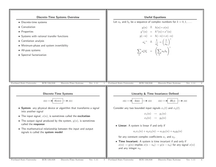
h ( n ) H ( z ) x ( n ) H [ x ( n )] y ( n ) x ( n ) y ( n ) x ( n ) - PowerPoint PPT Presentation

Discrete-Time Systems Overview Useful Equations Let a k and b k be a sequence of complex numbers for k = 0 , 1 , . . . . • Discrete-time systems • Convolution � y ( n ) h ( n ) ∗ x ( n ) y ∗ ( n ) h ∗ ( n ) ∗ x ∗ ( n ) • Properties = y ( − n ) = h ( − n ) ∗ x ( − n ) • Systems with rational transfer functions � 1 � ∗ 1 • Correlation analysis a −∗ � = k a ∗ a k • Minimum-phase and system invertibility k � ∗ �� • All-pass systems � a ∗ k b ∗ = a k b k k • Spectral factorization k k Portland State University ECE 538/638 Discrete-Time Systems Ver. 1.11 1 Portland State University ECE 538/638 Discrete-Time Systems Ver. 1.11 2 Discrete-Time Systems Linearity & Time Invariance Defined h ( n ) H ( z ) x ( n ) H [ x ( n )] y ( n ) x ( n ) y ( n ) x ( n ) y ( n ) • System : any physical device or algorithm that transforms a signal Consider any two bounded input signals x 1 ( t ) and x 2 ( t ) . into another signal x 1 ( n ) → y 1 ( n ) • The input signal, x ( n ) , is sometimes called the excitation x 2 ( n ) → y 2 ( n ) • The output signal produced by the system, y ( n ) , is sometimes called the response • Linear: A system is linear if and only if • The mathematical relationship between the input and output a 1 x 1 ( n ) + a 2 x 2 ( n ) → a 1 y 1 ( n ) + a 2 y 2 ( n ) signals is called the system model for any constant complex coefficients a 1 and a 2 . • Time Invariant: A system is time invariant if and only if x ( n ) → y ( n ) implies x ( n − n 0 ) → y ( n − n 0 ) for any signal x ( n ) and any integer n 0 . Portland State University ECE 538/638 Discrete-Time Systems Ver. 1.11 3 Portland State University ECE 538/638 Discrete-Time Systems Ver. 1.11 4

Justification of Scope Linear Time-Invariant (LTI) Systems • The assumption that a system is LTI and at rest may seem far too h ( n ) H ( z ) x ( n ) y ( n ) x ( n ) y ( n ) restrictive • In practice these assumptions are rarely justified • We shall limit our attention to linear systems • Nonetheless, these concepts provide an important and practically • In most cases, we will assume the systems are also time-invariant useful framework – This assumption can be relaxed with adaptive filters – Gives us a sense of what questions to ask about a system • Finally, we will assume the systems are always initially at rest – LTI theory is the basis of many non-LTI techniques • In this case, the impulse response completely characterizes the – In advanced courses nonlinear systems are sometimes treated system as time-varying systems (varying operating points) – Time-varying systems are a “simple” generalization of LTI δ ( n ) → h ( n ) theory – Assumption can often be weakened to slowly time-varying – Basis of adaptive filters and moving-window approaches Portland State University ECE 538/638 Discrete-Time Systems Ver. 1.11 5 Portland State University ECE 538/638 Discrete-Time Systems Ver. 1.11 6 LTI Systems: Convolution LTI Systems: Matrix Convolution � y (0) � � x (0) 0 0 � · · · h ( n ) H ( z ) x ( n ) y ( n ) x ( n ) y ( n ) y (1) x (1) x (0) 0 · · · � � � � � � � � � � � � . . . . ... . . . . � � � � ∞ ∞ . . . . � � � � y ( M − 2) x ( M − 2) x ( M − 3) 0 � � � � � � · · · y ( n ) = x ( n ) ∗ h ( n ) � x ( k ) h ( n − k ) = x ( n − k ) h ( k ) � � � � y ( M − 1) x ( M − 1) x ( M − 2) x (0) h (0) � � � � � � · · · � � � � k = −∞ k = −∞ y ( M ) x ( M ) x ( M − 1) x (1) h (1) � � � � · · · � � � � � � = � � � � � � . . . . � . � ... � � � � . . . . . � � • Here ∗ denotes convolution � . � � . . . � . � y ( N − 1) � � x ( N − 1) x ( N − 2) x ( N − M ) � h ( M − 1) · · · � � � � � y ( N ) � � 0 x ( N − 1) x ( N − M + 1) � • If x ( n ) and h ( n ) are finite duration , this can also be expressed in · · · � � � � � � � � matrix notation � . � � . . . � ... . . . . � � � � . . . . – Let x ( n ) be nonzero only for 0 ≤ n ≤ N − 1 � � � � y ( L − 2) 0 0 x ( N − 2) � � � · · · � y ( L − 1) 0 0 x ( N − 1) – Let h ( n ) be nonzero only for 0 ≤ n ≤ M − 1 such that M < N · · · X ∈ C L × M – Then y ( n ) is nonzero only for 0 ≤ n ≤ L − 1 y = Xh – L � N + M − 1 Note that all the elements along any diagonal of X are equal Portland State University ECE 538/638 Discrete-Time Systems Ver. 1.11 7 Portland State University ECE 538/638 Discrete-Time Systems Ver. 1.11 8

LTI Systems: Matrix Convolution LTI Systems: Matrix Convolution y (0) h (0) 0 0 0 � � � � y = Xh y = Hx · · · y (1) h (1) h (0) 0 0 · · · � � � � � � � � � x (0) � . . . . . � � � ... � . . . . . � � � � . . . . . x (1) � � � � y ( M ) h ( M − 1) h ( M − 2) 0 0 � � • X ∈ C L × M is called the input data matrix � � � � · · · � � � � � � y ( M + 1) 0 h ( M − 1) 0 0 � � . � � � · · · � � . � � � � � . y ( M + 2) 0 0 0 0 � � • It is a Toeplitz matrix since the diagonal elements are equal � � � · · · � x ( M ) � � � � � � � � � � � � = x ( M + 1) . . . . . � � ... � � � � • Note also that the first and last M − 1 rows contain zero values . . . . . � � � � � � . . . . . x ( M + 2) � � � � � � y ( N − 2) 0 0 h (0) 0 � � · · · that are outside the range of x ( n ) � � � � � � � y ( N − 1) � � 0 0 h (1) h (0) � . � � · · · � � � � . � � � y ( N ) � � 0 0 h (2) h (1) � . • Thus the first and last M − 1 samples of y ( n ) contain boundary � � · · · x ( N − 2) � � � � � � � � � � effects x ( N − 1) � � � � . . . . . ... � . � � . . . . � . . . . . � � � � y ( L − 2) 0 0 h ( M ) h ( M − 1) � � � � · · · y ( L − 1) 0 0 0 h ( M ) · · · H ∈ C L × N y = Hx Note that all the elements along any diagonal of X are equal Portland State University ECE 538/638 Discrete-Time Systems Ver. 1.11 9 Portland State University ECE 538/638 Discrete-Time Systems Ver. 1.11 10 LTI Systems: Stability LTI Systems: Causality h ( n ) H ( z ) x ( n ) y ( n ) x ( n ) y ( n ) h ( n ) H ( z ) x ( n ) y ( n ) x ( n ) y ( n ) • There are many definitions of stability • Causal : A system in which y ( n ) depends only on present and/or • The most common is BIBO stability past values of x ( n ) • BIBO Stability : A system is called bounded-input • Note that we can implement non-causal discrete-time systems bounded-output (BIBO) stable if every bounded input produces off-line if the entire input signal is known before the output must a bounded output be calculated | x ( n ) | < ∞ for all n → | y ( n ) | < ∞ for all n • An LTI system is causal iff h ( n ) is causal: • An equivalent condition for LTI systems is h ( n ) = 0 for n < 0 ∞ • This in turn implies that the ROC of H ( z ) includes | z | = ∞ � | h ( n ) | < ∞ • Thus, LTI systems that are causal and stable have an ROC that n = −∞ ranges from inside the unit circle to | z | = ∞ • Note that this is a sufficient and necessary (proof?) condition for the ROC of H ( z ) to include the unit circle Portland State University ECE 538/638 Discrete-Time Systems Ver. 1.11 11 Portland State University ECE 538/638 Discrete-Time Systems Ver. 1.11 12