Grouping and Edges Computer Vision Fall 2018 Columbia University - PowerPoint PPT Presentation
Grouping and Edges Computer Vision Fall 2018 Columbia University Homework 2 Posted online Monday Due October 8 before class starts no exceptions! Get started early covers material up to today Image Gradients Review First
Grouping and Edges Computer Vision Fall 2018 Columbia University
Homework 2 • Posted online Monday • Due October 8 before class starts — no exceptions! • Get started early — covers material up to today
Image Gradients Review
First Derivative ∂ I * [ − 1,1] = ∂ x ∂ I * [ − 1,1] T = ∂ y
Second Derivative ∂ 2 I * [ − 1,1] = ∂ x 2 ∂ 2 I * [ − 1,1] T = ∂ y 2
Image Gradients Source: Seitz and Szeliski
What is an edge? Source: G Hager
What about noise? Source: G Hager
Handling Noise • Filter with a Gaussian to smooth, then take gradients • But, convolution is linear Gaussian Filter Laplacian Filter * [ − 1,1] * [ − 1,1] = * [ − 1,1] T * [ − 1,1] T =
Edges
Why do we care about edges? • Extract information • Recognize objects Vertical vanishing • Help recover geometry point Vanishing and viewpoint (at infinity) line Vanishing Vanishing point point
Origin of Edges surface normal discontinuity depth discontinuity surface color discontinuity illumination discontinuity • Edges are caused by a variety of factors Source: Steve Seitz
Low-level edges vs. perceived contours Shadows Background Texture
Kanizsa Triangle
Low-level edges vs. perceived contours human segmentation image gradient magnitude Berkeley segmentation database: http://www.eecs.berkeley.edu/Research/Projects/CS/vision/grouping/segbench/ Source: L. Lazebnik
Berkeley Segmentation Data Set Credit: David Martin David Martin, Charless Fowlkes, Doron Tal, Jitendra Malik
Learn from humans which combination of features is most indicative of a “good” contour? Human-marked segment boundaries [D. Martin et al. PAMI 2004]
What features are responsible for perceived edges? Feature profiles (oriented energy, brightness, color, and texture gradients) along the patch’s horizontal diameter [D. Martin et al. PAMI 2004] Kristen Grauman, UT-Austin
What features are responsible for perceived edges? Feature profiles (oriented energy, brightness, color, and texture gradients) along the patch’s horizontal diameter [D. Martin et al. PAMI 2004] Kristen Grauman, UT-Austin
Credit: David Martin
[D. Martin et al. PAMI 2004] Kristen Grauman, UT-Austin
Contour Detection Canny+opt thresholds Human agreement Canny Prewitt, Learned Sobel, with Roberts combined features Source: Jitendra Malik: http://www.cs.berkeley.edu/~malik/ malik-talks-ptrs.html
Canny Edge Detector Widely used edge detector John Canny’s masters thesis
Demonstrator Image
Canny edge detector 1. Filter image with x, y derivatives of Gaussian Source: D. Lowe, L. Fei-Fei
Derivative of Gaussian filter x -direction y -direction
Compute Gradients X Derivative of Gaussian Y Derivative of Gaussian (x2 + 0.5 for visualization)
Canny edge detector 1. Filter image with x, y derivatives of Gaussian 2. Find magnitude and orientation of gradient Source: D. Lowe, L. Fei-Fei
Compute Gradient Magnitude sqrt( XDerivOfGaussian .^2 + YDerivOfGaussian .^2 ) = gradient magnitude (x4 for visualization)
Compute Gradient Orientation • Threshold magnitude at minimum level • Get orientation via theta = atan2(gy, gx)
Canny edge detector 1. Filter image with x, y derivatives of Gaussian 2. Find magnitude and orientation of gradient 3. Non-maximum suppression: – Thin multi-pixel wide “ridges” to single pixel width Source: D. Lowe, L. Fei-Fei
Non-maximum suppression for each orientation At pixel q: We have a maximum if the value is larger than those at both p and at r. Interpolate along gradient direction to get these values. Source: D. Forsyth
Before Non-max Suppression Gradient magnitude (x4 for visualization)
After non-max suppression Gradient magnitude (x4 for visualization)
Canny edge detector 1. Filter image with x, y derivatives of Gaussian 2. Find magnitude and orientation of gradient 3. Non-maximum suppression: – Thin multi-pixel wide “ridges” to single pixel width 4. ‘Hysteresis’ Thresholding Source: D. Lowe, L. Fei-Fei
Edge linking Assume the marked point is an edge point. Then we construct the tangent to the edge curve (which is normal to the gradient at that point) and use this to predict the next points (here either r or s). Source: D. Forsyth
‘Hysteresis’ thresholding • Two thresholds – high and low • Grad. mag. > high threshold? = strong edge • Grad. mag. < low threshold? noise • In between = weak edge • ‘Follow’ edges starting from strong edge pixels • Continue them into weak edges Connected components (Szeliski 3.3.4) • Source: S. Seitz
Final Canny Edges 𝜏 = 2, 𝑢 𝑚𝑝𝑥 = 0.05, 𝑢 h 𝑗 h = 0.1
Effect of σ (Gaussian kernel spread/size) Original 𝜏 = 2 𝜏 = 4 2 The choice of σ depends on desired behavior • large σ detects large scale edges • small σ detects fine features Source: S. Seitz
Fitting
Fitting • Want to associate a model with observed features [Fig from Marszalek & Schmid, 2007] For example, the model could be a line, a circle, or an arbitrary shape. Slide credit: K. Grauman
Case study: Line fitting • Why fit lines? Many objects characterized by presence of straight lines • Wait, why aren’t we done just by running edge detection? Slide credit: K. Grauman
Difficulty of line fitting • Extra edge points (clutter), multiple models: – which points go with which line, if any? • Only some parts of each line detected, and some parts are missing: – how to find a line that bridges missing evidence? • Noise in measured edge points, orientations: – how to detect true underlying parameters? Slide credit: K. Grauman
Fitting: Main idea • Choose a parametric model to represent a set of features • Membership criterion is not local • Can’t tell whether a point belongs to a given model just by looking at that point • Three main questions: • What model represents this set of features best? • Which of several model instances gets which feature? • How many model instances are there? • Computational complexity is important • It is infeasible to examine every possible set of parameters and every possible combination of features Slide credit: L. Lazebnik
Fitting lines: Hough transform • Given points that belong to a line, what is the line? • How many lines are there? • Which points belong to which lines? • Hough Transform is a voting technique that can be used to answer all of these questions. Main idea: 1. Record vote for each possible line on which each edge point lies. 2. Look for lines that get many votes .
Finding lines in an image: Hough space y b b 0 m 0 x m image space Hough (parameter) space Connection between image (x,y) and Hough (m,b) spaces • A line in the image corresponds to a point in Hough space • To go from image space to Hough space: – given a set of points (x,y), find all (m,b) such that y = mx + b Slide credit: Steve Seitz
Finding lines in an image: Hough space y b y 0 x 0 x m image space Hough (parameter) space Connection between image (x,y) and Hough (m,b) spaces • A line in the image corresponds to a point in Hough space • To go from image space to Hough space: – given a set of points (x,y), find all (m,b) such that y = mx + b • What does a point (x 0 , y 0 ) in the image space map to? – Answer: the solutions of b = -x 0 m + y 0 – this is a line in Hough space Slide credit: Steve Seitz
Finding lines in an image: Hough space y b ( x 1 , y 1 ) y 0 ( x 0 , y 0 ) b = – x 1 m + y 1 x 0 x m image space Hough (parameter) space What are the line parameters for the line that contains both (x 0 , y 0 ) and (x 1 , y 1 )? • It is the intersection of the lines b = –x 0 m + y 0 and b = –x 1 m + y 1
Finding lines in an image: Hough algorithm y b x m image space Hough (parameter) space How can we use this to find the most likely parameters (m,b) for the most prominent line in the image space? • Let each edge point in image space vote for a set of possible parameters in Hough space • Accumulate votes in discrete set of bins*; parameters with the most votes indicate line in image space.
Hough transform algorithm Using the polar parameterization: H: accumulator array (votes) x cos y sin d θ − θ = Basic Hough transform algorithm d 1. Initialize H[d, θ ]=0 2. for each edge point I[x,y] in the image for θ = [ θ min to θ max ] // some quantization θ d x cos y sin = θ − θ H[d, θ ] += 1 3. Find the value(s) of (d, θ ) where H[d, θ ] is maximum 4. The detected line in the image is given by d x cos y sin = θ − θ Time complexity (in terms of number of votes per pt)? Source: Steve Seitz
Recommend
More recommend
Explore More Topics
Stay informed with curated content and fresh updates.
