EDGE DETECTION INEL 6088 - Computer Vision Davies Ch. 5, Jain et. - PowerPoint PPT Presentation
EDGE DETECTION INEL 6088 - Computer Vision Davies Ch. 5, Jain et. al. Ch. 5 Sec. 4.2 Szelinski ideal ~real 2 Edge point point at which the local intensity changes significantly Edge fragment edge (point) and orientation Edge
EDGE DETECTION INEL 6088 - Computer Vision Davies Ch. 5, Jain et. al. Ch. 5 Sec. 4.2 Szelinski
ideal ~real 2
Edge point – point at which the local intensity changes significantly Edge fragment – edge (point) and orientation Edge detector – produces a set of edges (points or fragments) Edge linking – orders a list of edges Contour – list of edges Edge following – searching the (input) image to determine contours
Real image Edge detector produces: • correct edges • false edges (false positives) • can miss edges (false negatives) 4
EDGE DETECTION USING GRADIENT Simple way G[f(x,y)]=[G x G y ] T G x = δ f/ δ x ≈ f[i,j+1]-f[i,j] « gradient at [i, j+ ½ ] G y = δ f/ δ y ≈ f[i+1,j]-f[i,j] « gradient at [i+ ½ , j] To get the gradient at the same point [i+ ½ , j+ ½ ], use: 5
j Steps: • filtering i • enhancement • detection • sometimes, localisation Roberts: P5 = |P5 - P9| + |P8 – P6| Sobel: c = mult. by 2 Prewitt: Sobel with c = 1 6
1 1 � � F r,c = f r,c ∗ g r,c = f i,j g r − i,c − j 2 1 15 33 29 i = − 1 j = − 1 3 2 11 28 60 C = 5 25 32 40 41 g x =conv2(C,S y ) = 4 20 33 43 41 2 5 19 64 110 91 29 3 8 18 52 127 148 60 4 2 19 27 35 3 30 68 65 43 31 12 2 22 60 77 33 -23 -19 -1 -25 -60 -62 -45 -25 -6 1 2 1 -5 -30 -78 -129 -160 -125 -41 -4 -10 -27 -67 -108 -97 -35 0 0 0 S y = -1 -2 -1 5 + 2*25 + 32 - (2 + 2 + 15) = 68
2 1 13 32 14 -33 -29 S x = S y ’ 7 4 34 90 77 -94 -118 13 30 56 99 121 -129 -190 g y =conv2(S y , C)= 18 72 90 79 75 -151 -183 19 67 98 86 41 -153 -158 13 24 58 73 40 -97 -111 4 2 15 25 16 -27 -35 G(i,j)=sqrt(g x2 + g y2 ) 2.8284 5.0990 23.0217 71.5542 110.8873 96.7988 41.0122 7.6158 8.9443 38.4708 103.9423 148.5194 175.3283 132.3782 13.3417 42.4264 88.0909 118.4314 128.4134 132.6725 190.3786 18.1108 75.2861 108.1665 110.3177 81.9390 152.7416 183.9837 19.0263 71.5122 114.9087 106.0189 60.8769 155.0290 158.1139 13.9284 38.4187 97.2008 148.2228 164.9242 158.2214 118.3300 5.6569 10.1980 30.8869 71.5122 109.1788 100.6876 49.4975
uint8 version of G= 3 5 23 72 111 97 41 8 9 38 104 149 175 132 13 42 88 118 128 133 190 18 75 108 110 82 153 184 19 72 115 106 61 155 158 14 38 97 148 165 158 118 6 10 31 72 109 101 49 Using a threshold of 0.4 to detect the edge: 0 0 0 0 1 0 0 0 0 0 1 1 1 1 0 0 0 1 1 1 1 0 0 1 1 0 1 1 0 0 1 1 0 1 1 0 0 0 1 1 1 1 0 0 0 0 1 0 0
Filtered with 7x7 gaussian filter 10
unfiltered 11
Filtered, noisy 12
Unfiltered, noisy 13
EDGE DETECTORS THAT USE THE SECOND DERIVATIVE Change in sign indicates edge Two ways: • Laplacian • Second directional derivative 14
LAPLACIAN Combined to get Also used: 15
16
17
SECOND DIRECTIONAL DERIVATIVE � Second derivative computed in the direction of the gradient � Implement using the formula: 18
Problem with Laplacian and second-derivative-operator: • very sensitive to noise • small peaks in first derivative produce zero- crossing in the second derivative. Solution: Filter out noise before edge enhancement Laplacian of Gaussian (LoG) Smoothing: Gaussian smoothing � Enhancement: Second-derivative edge enhancement � Detection: zero-crossing in the second derivative with a corresponding � large peak (i.e. above some threshold) in the first derivative If desired, use linear interpolation to locate the edge with sub-pixel � resolution 19
The output of the LoG operator, h(x,y) is given by: h ( x, y ) = r 2 [ g ( x, y ) ? f ( x, y )] Mexican-hat h ( x, y ) = [ r 2 g ( x, y )] ? f ( x, y ) Operator r 2 g ( x, y ) = x 2 + y 2 � 2 � 2 � x 2 + y 2 ✓ ◆ exp � 4 2 � 2 20
Two ways of doing LoG: • Gaussian smoothing followed by laplacian • Convolution of image with a linear filter that is the laplacian of a gaussian filter To obtain real edges, it might be necessary to combine information from filters of different sizes. The problem of combining edges obtained from different size operators still remains. 21
22
LoG Results Smoothing causes blurring large σ : better noise filtering but more blurring – can cause edge merging By applying filters of different sizes and analysing the results, better edge detection can be accomplished. 23
An alternative approach is to fit a function to the image and then detect the edges in the function… 24
Facet model: fit a function only in the local neighborhood of each pixel. 25
Example: bicubic polynomial 26
Masks for computing the coefficients of the bicubic approximation. 27
28
∂ f ∂ x cos θ + ∂ f f 0 θ ( x, y ) = ∂ y sin θ ∂ 2 f ∂ x 2 cos 2 θ + 2 ∂ 2 f ∂ x ∂ y cos θ sin θ + ∂ 2 f ∂ y 2 sin 2 θ f 00 θ ( x, y ) = k 3 The angle may be chosen to be sin θ = the angle of the approximating p k 2 2 + k 2 3 plane: k 2 cos θ = p k 2 2 + k 2 3 θ ( x 0 , y 0 ) = 2(3 k 7 cos 2 θ + 2 k 8 sin θ cos θ + k 9 sin 2 θ ) x 0 f 00 +2( k 8 cos 2 θ + 2 k 9 sin θ cos θ + 3 k 10 sin 2 θ ) y 0 +2( k 4 cos 2 θ + k 5 sin θ cos θ + k 6 sin 2 θ ) 29
x 0 = ρ cos θ = ρ sin θ y 0 6( k 10 sin 3 θ + k 9 sin 2 θ cos θ + k 8 sin θ cos 2 θ + k 7 cos 3 θ ) ρ f 00 θ ( x 0 , y 0 ) = +2( k 6 sin 2 θ + k 5 sin θ cos θ + k 4 cos 2 θ ) = A ρ + B There is an edge at (x 0 ,y 0 ) if for some ρ , | ρ |< ρ 0 where ρ 0 is the length of the side of a pixel, f θ ”(x 0 ,y 0 ; ρ ) = 0 and f θ ’(x 0 ,y 0 ; ρ ) ≠ 0 30
31
32
CANNY EDGE DETECTION � Let I[i,j] be the image. First use Gaussian smoothing: S[i,j]=G[i,j; σ ]*I[i,j] � Find approx. gradient using 2 × 2 first-diff. approx. � x direction: P[i,j]=(S[i,j+1]-S[i,j]+S[i+1,j+1]-S[i+1,j])/2 � y direction: Q[i,j]=(S[i,j]-S[i+1,j]+S[i,j+1]-S[i+1,j+1])/2 33
CANNY EDGE DETECTION (CONT) � Magnitude and orientation: rectangular to polar conversion: � M[I,j]= √ (P[i,j] 2 +Q[i,j] 2 ) � θ [i,j] = arctan(Q[i,j]/P[i,j]) � Non-maxima Suppression � Thins the ridges of gradient magnitude to one pixel � Passes a 3x3 neighborhood across the magnitude array M[I,j] and replace pixels with 0 if not greater than neighbors 34
Possible gradient orientations are partitioned into the following sectors for non-maxima suppression 1 2 3 4 0 5 6 7 8 Replace pixel 0 with value 0 if it is not bigger than neighboring pixels in the (quantized) direction of the gradient 35
CANNY EDGE DETECTION (CONT) � Thresholding � Apply two threshold t 1 and t 2 , with t 2 = 2*t 1 � This produces two threshold images T 1 & T 2 � T 2 will have fewer edges, but might have gaps � When the end of a contour in T 2 is reached, look into T 1 at the 8-neighboring locations to see if there are further edge points that can be linked to the contour. 36
Test Image (256x256) 37
Canny with 7x7 Gaussian smoothing + gradient approx + NMS 38
Canny with 31x31 Gaussian smoothing 39
SEQUENTIAL METHODS � Edge following: � scan image looking for strong edge � extend the edge in the proper direction by looking at neighboring edges � link if directions are compatible � look at large neighborhood to fill in missing edges 40
41
Corner Detection Consider the spatial image gradient, [ E x , E y ] T (the subscripts indicate par- ∂ E tial di ff erentiation, e.g. E x = ∂ x ). Consider a generic image point p and a neighborhood Q of p , and a matrix C defined as ✓ P E 2 P E x E y ◆ P E x E y P E 2 x C = y where the sums are taken over Q . A rotation of the coordinate axes can diago- nalized the matrix, ✓ ◆ 0 λ 1 C = 0 λ 2 • λ 1 ' λ 2 ' 0: gradient vanishes everywhere • λ 1 > 0; λ 2 ' 0: Q contains an ideal step edge; eigenvector associated with λ 1 gives the direction of the edge • λ 1 > 0; λ 2 > 0: Q contains a corner. The larger the lambda ’s the stronger the edges.
Corner detection algorithm • Inputs: grayscale image I and two parameters: – threshold t on λ 2 (smallest eigenvalue) – size N of square window (neighborhood), 2 N + 1 • Compute gradient over entire image • For each image point p , 1. form matrix C over a (2 N × 1) × (2 N × 1) neighborhood Q of p 2. find λ 2 3. if λ 2 ≥ t , save the coordinates of p into a list L • Sort L in decreasing order of λ 2 • Scan L and for each point p delete other points in L that belong to Q .
Recommend
More recommend
Explore More Topics
Stay informed with curated content and fresh updates.
