C18 Computer Vision Lecture 6 Salient feature detection: points, - PowerPoint PPT Presentation
C18 Computer Vision Lecture 6 Salient feature detection: points, edges and SIFTs Victor Adrian Prisacariu http://www.robots.ox.ac.uk/~victor Computer Vision: This time 5. Imaging geometry, camera calibration. 6. 6. Sa Salie lient
C18 Computer Vision Lecture 6 Salient feature detection: points, edges and SIFTs Victor Adrian Prisacariu http://www.robots.ox.ac.uk/~victor
Computer Vision: This time… 5. Imaging geometry, camera calibration. 6. 6. Sa Salie lient feature detectio ion and desc scrip iptio ion. 1. Cameras as photometric devices (just a note) 2. Image convolution (in the context of image derivatives). 3. Edge detection. 4. Corner detection. 5. SIFT + LIFT. 7. Recovering 3D from two images I: epipolar geometry. 8. Recovering 3D from two images II: stereo correspondences, triangulation, neural nets.
Feature points are useful …
6.1 Cameras as Photometric Devices • In Lecture 5, we considered the camera as a geometric abstraction ground on the rectilinear propagation of light. • But they are also photometric devices. • Important to consider the way image formation depends on: – The nature of the scene surface (reflecting, absorbing). – The relative orientations of the surface, light source and cameras. – The power and spectral properties of the source. – The spectral properties of the imaging system. • The important overall outcome (e.g. Forsyth & Ponce, p62) is that imag age irr rradia iance is s pr prop oportio ional l to o sce scene rad adia iance. • A relief! This means the image really can tell us about the scene.
6.1 Cameras as Photometric Devices • But the study of photometry (often called physics-based vision) requires detailed models of reflectance properties of the scene and the imaging process itself. • E.g. understanding (or learning) how light scatters on water droplets allowed this image to de-fogged. • Can we avoid such detail when aiming to get geometry? … Yes – by considering aspects of scene geometry that are step ch changes in or in invariant to image irradiance.
Step irradiance changes are due to … • Changes in Scene Radiance: – Natural (e.g. shadows) or deliberately introduced via artificial illumination. • Changes in scene reflectance at sudden changes in surface orientation: – Arise at the intersection of two surfaces, so represent geometrical entities fixed on the object. • Changes in reflectance properties due to changes in surface albedo: – Reflectance properties are scaled by a changing albedo arising from surface markings. Also fixed to the object.
6.2 Feature detection • We are looking for step sp spatial l ch changes in image irradiance because: – They are likely to be tied to scene geometry; – They are likely to be salient (have high info content) • A simple classification of changes in image irradiance 𝐽(𝑦, 𝑧) is into areas that, locally, have 1D structure 2D structure Edge De Detectors Cor Corner De Detectors
Image operations for Feature Detection • Feature detection is often a loc local op operation, working without knowledge of higher geometrical entities or objects (this is changing nowadays …) • We use pixel values 𝐽(𝑦, 𝑧) and derivatives 𝜖𝐽/𝜖𝑦 and 𝜖𝐽/𝜖𝑧 . • It is useful to have a non on-directional com ombination of these, so that a feature map of a rotated image is identical to the rotated feature map of the original image. • Considering edge detection, two possibilities are: – Search for maxima in the gradient magnitude 2 2 𝜖𝐽 𝜖𝐽 - 1 st order, but non-linear + 𝜖𝑦 𝜖𝑧 – Search for zeros in the Laplacian 𝜖 2 𝐽 𝜖 2 𝐽 𝜖𝑧 2 - linear, but 2 nd order 𝛼 2 𝐽 = 𝜖𝑦 2 +
Which to chose? • The gradient t magnitu tude is attractive because it is first order in the derivatives . Differentiation enhances noise, and the 2nd derivatives in the Laplacian operator introduces even more. • The Laplacian is attractive because it is linear , which means it can be implemented by a succession of fast linear operations -- effectively matrix operations as we are dealing with a pixelated image. • Both th approaches s have been use sed. • For both approaches we need to consider: – How to compute the gradients, and – How to suppress noise (so that insignificant variations in pixel intensity are not flagged as edges).
Preamble: Spatial Convolution • You are familiar with the 1D con onvolu lution in inter ergral in the time domain between an input signal 𝑗(𝑢) and im ction ℎ(𝑢) . impulse res esponse fu funct +∞ +∞ 𝑝 𝑢 = 𝑗 𝑢 ∗ ℎ 𝑢 = න 𝑗 𝑢 − 𝜐 ℎ 𝜐 d𝜐 = න 𝑗 𝜐 ℎ 𝑢 − 𝜐 d𝜐 −∞ −∞ • The second equality reminds us that convolution commutes 𝑗 𝑢 ∗ ℎ 𝑢 = ℎ 𝑢 ∗ 𝑗(𝑢) . It also associates. • In the frequency domain we would write 𝑃 𝑡 = 𝐼 𝑡 𝐽(𝑡) . • Now in the continuous 2D domain, the spatia tial con onvolution in integ egral is: +∞ +∞ 𝑝 𝑦, 𝑧 = 𝑗 𝑦, 𝑧 ∗ ℎ(𝑦, 𝑧) න න 𝑗 𝑦 − 𝑏, 𝑧 − 𝑐 ℎ 𝑏, 𝑐 d𝑏d𝑐 −∞ −∞ • In the spatial domain you’ll often see ℎ(𝑦, 𝑧) referred as the poin oint t spread fu funct ction, the con onvolu luti tion mask or the con onvolution kern ernel.
Discrete Spatial Convolution • For pixelated images 𝐽(𝑦, 𝑧) , we need a dis iscrete con onvoluti tion: 𝑃 𝑦, 𝑧 = 𝐽 𝑦, 𝑧 ∗ ℎ 𝑦, 𝑧 = 𝐽 𝑦 − 𝑗, 𝑧 − 𝑘 ℎ(𝑗, 𝑘) 𝑗 𝑘 for 𝑦, 𝑧 ranging over the image width and height respectively, and 𝑗, 𝑘 ensuring access is made to any and all non-zero entries in h . Many authors rewrite the convolution by replacing ℎ(𝑗, 𝑘) with ത • ℎ −𝑗, −𝑘 𝑃 𝑦, 𝑧 = ∑∑𝐽 𝑦 − 𝑗, 𝑧 − 𝑘 ℎ 𝑗, 𝑘 = ∑∑𝐽 𝑦 + 𝑗, 𝑧 + 𝑘 ℎ −𝑗, −𝑘 = ∑∑𝐽 𝑦 + 𝑗, 𝑧 + 𝑗 ത ℎ 𝑗, 𝑘 This looks more like the expression for cross-correlation but, confusingly, it is still called convolution.
Computing partial derivatives using convolution • We can approximate 𝜖𝐽/𝜖𝑦 at image pixel (𝑦, 𝑧) using ce centr tral fi finit ite dif difference. 𝜖𝑦 ≈ 1 𝜖𝐽 𝐽 𝑦 + 1, 𝑧 − 𝐽 𝑦, 𝑧 + 𝐽 𝑦, 𝑧 − 𝐽 𝑦 − 1, 𝑧 = 2 = 1 2 𝐽 𝑦 + 1, 𝑧 − 𝐽 𝑦 − 1, 𝑧 • Writing this as a “proper” convolution would set: ℎ −1 = + 1 ℎ 1 = − 1 ℎ 0 = 0 2 2 1 𝐸 𝑦, 𝑧 = 𝐽 𝑦, 𝑧 ∗ ℎ 𝑦 = 𝐽 𝑦 − 𝑗, 𝑧 ℎ(𝑗) 𝑗=−1 • Notice how the “proper” mask is revered from what we might naively expect from the expression.
Computing partial derivatives using convolution 𝜖𝐽 1 • 𝜖𝑦 ≈ 2 𝐽 𝑦 + 1, 𝑧 − 𝐽 𝑦 − 1, 𝑧 Now, as ever: • Writing this as a “sort of correlation” ℎ −1 = − 1 ℎ 1 = + 1 ത ത ത ℎ 0 = 0 2 2 1 𝐸 𝑦, 𝑧 = 𝐽 𝑦, 𝑧 ∗ ത 𝐽 𝑦 + 𝑗, 𝑧 ത ℎ 𝑦 = ℎ(𝑗) 𝑗=−1 • Note how we can just lay this mask directly on the pixels to be multiplied and summed …
Example Results 𝐽(𝑦, 𝑧) x- gradient “image” y- gradient “image”
In 2 dimensions: • As before, one imagines the flipped “correlation - like” mask centered on the pixel, and the sum of the products completed • Often a 2D mask is “ sep eparable le ” in that it can be broken up into two separate 1D convolutions in 𝑦 and 𝑧 : 𝑃 = ℎ 2𝑒 ∗ 𝐽 = 𝑔 𝑧 ∗ 𝑦 ∗ 𝐽 • The computational complexity is lower, but intermediate storage is required, so for a small mask it might be cheaper to use it directly.
Example result – Laplacian (not-directional) The actual image is used grey- Laplacian level, not colour
Preamble: Noise and Smoothing • Dif ifferentia iatio ion en enhances no nois ise – the edge appears clear enough in images, but less so in the gradient map. • If we know the noise spectrum, we might find an optimal brickwall filter (𝑦, 𝑧) ↔ 𝐻(𝑡) to suppress noise edges outside the signal edge band. • But a sharp cut-off in spatial-frequency requires a wide spatial 𝑦, 𝑧 - an Infinite Impulse Response filter – not doable. • Can we compromise spread in space and signal-frequency in some optimal way?
Compromise in space and spatial-frequency • Suppose IR function is ℎ(𝑦) and ℎ ⇌ 𝐼 is a Fourier transform pair. • Define the spreads in space and spatial-frequency as 𝑌 and Ω where: ∫ 𝑦−𝑦 𝑛 2 ℎ 2 𝑦 𝑒𝑦 ∫ 𝑦 ℎ 2 𝑦 𝑒𝑦 𝑌 2 = with 𝑦 𝑛 = ∫ ℎ 2 𝑦 𝑒𝑦 ∫ ℎ 2 𝑦 𝑒𝑦 ∫ 𝜕−𝜕 𝑛 2 𝐼 2 𝜕 𝑒𝜕 ∫ 𝜕𝐼 2 𝜕 𝑒𝜕 Ω 2 = with 𝜕 𝑛 = ∫ 𝐼 2 𝜕 𝑒𝜕 ∫ 𝐼 2 𝜕 𝑒𝜕 • Now vary ℎ to minimize the product of the spreads 𝑉 = 𝑌Ω . • An uncertainty principle indicates that 𝑉 𝑛𝑗𝑜 = 1/2 when: 𝑦 2 1 ℎ 𝑦 = a 2𝜌𝜏 exp(− 𝜏 2 ) a Gaussian fu functi tion =
6.3 Edge Detection: Simple Approach: Sobel • Convolve with kernels: −1 0 1 −1 −2 −1 ℎ 𝑦 = and ℎ 𝑧 = −2 0 2 0 0 0 −1 0 1 1 2 1 • Compute magnitudes: 2 𝐽 ∗ ℎ 𝑦 2 + 𝐽 ∗ ℎ 𝑧 edge map = • (optionally) smooth.
Recommend
More recommend
Explore More Topics
Stay informed with curated content and fresh updates.
