Greedy Algorithms Lecture 19 April 4, 2017 Chandra Chekuri (UIUC) - PowerPoint PPT Presentation
CS 374: Algorithms & Models of Computation, Spring 2017 Greedy Algorithms Lecture 19 April 4, 2017 Chandra Chekuri (UIUC) CS374 1 Spring 2017 1 / 1 Part I Greedy Algorithms: Tools and Techniques Chandra Chekuri (UIUC) CS374 2
CS 374: Algorithms & Models of Computation, Spring 2017 Greedy Algorithms Lecture 19 April 4, 2017 Chandra Chekuri (UIUC) CS374 1 Spring 2017 1 / 1
Part I Greedy Algorithms: Tools and Techniques Chandra Chekuri (UIUC) CS374 2 Spring 2017 2 / 1
What is a Greedy Algorithm? Chandra Chekuri (UIUC) CS374 3 Spring 2017 3 / 1
What is a Greedy Algorithm? No real consensus on a universal definition. Chandra Chekuri (UIUC) CS374 3 Spring 2017 3 / 1
What is a Greedy Algorithm? No real consensus on a universal definition. Greedy algorithms: make decision incrementally in small steps without backtracking 1 decision at each step is based on improving local or current state 2 in a myopic fashion without paying attention to the global situation decisions often based on some fixed and simple priority rules 3 Chandra Chekuri (UIUC) CS374 3 Spring 2017 3 / 1
Pros and Cons of Greedy Algorithms Pros: Usually (too) easy to design greedy algorithms 1 Easy to implement and often run fast since they are simple 2 Several important cases where they are effective/optimal 3 Lead to a first-cut heuristic when problem not well understood 4 Chandra Chekuri (UIUC) CS374 4 Spring 2017 4 / 1
Pros and Cons of Greedy Algorithms Pros: Usually (too) easy to design greedy algorithms 1 Easy to implement and often run fast since they are simple 2 Several important cases where they are effective/optimal 3 Lead to a first-cut heuristic when problem not well understood 4 Cons: Very often greedy algorithms don’t work. Easy to lull oneself 1 into believing they work Many greedy algorithms possible for a problem and no 2 structured way to find effective ones Chandra Chekuri (UIUC) CS374 4 Spring 2017 4 / 1
Pros and Cons of Greedy Algorithms Pros: Usually (too) easy to design greedy algorithms 1 Easy to implement and often run fast since they are simple 2 Several important cases where they are effective/optimal 3 Lead to a first-cut heuristic when problem not well understood 4 Cons: Very often greedy algorithms don’t work. Easy to lull oneself 1 into believing they work Many greedy algorithms possible for a problem and no 2 structured way to find effective ones CS 374: Every greedy algorithm needs a proof of correctness Chandra Chekuri (UIUC) CS374 4 Spring 2017 4 / 1
Greedy Algorithm Types Crude classification: Non-adaptive: fix some ordering of decisions a priori and stick 1 with the order Adaptive: make decisions adaptively but greedily/locally at each 2 step Chandra Chekuri (UIUC) CS374 5 Spring 2017 5 / 1
Greedy Algorithm Types Crude classification: Non-adaptive: fix some ordering of decisions a priori and stick 1 with the order Adaptive: make decisions adaptively but greedily/locally at each 2 step Plan: See several examples 1 Pick up some proof techniques 2 Chandra Chekuri (UIUC) CS374 5 Spring 2017 5 / 1
Part II Scheduling Jobs to Minimize Average Waiting Time Chandra Chekuri (UIUC) CS374 6 Spring 2017 6 / 1
The Problem n jobs J 1 , J 2 , . . . , J n . J i has non-negative processing time p i One server/machine/person available to process jobs. Schedule/order the jobs to minimize total or average waiting time Waiting time of J i in schedule σ : sum of processing times of all jobs scheduled before J i J 1 J 2 J 3 J 4 J 5 J 6 time 3 4 1 8 2 6 Chandra Chekuri (UIUC) CS374 7 Spring 2017 7 / 1
The Problem n jobs J 1 , J 2 , . . . , J n . J i has non-negative processing time p i One server/machine/person available to process jobs. Schedule/order the jobs to minimize total or average waiting time Waiting time of J i in schedule σ : sum of processing times of all jobs scheduled before J i J 1 J 2 J 3 J 4 J 5 J 6 time 3 4 1 8 2 6 Example: schedule is J 1 , J 2 , J 3 , J 4 , J 5 , J 6 . Total waiting time is 0 + 3 + (3 + 4) + (3 + 4 + 1) + (3 + 4 + 1 + 8) + . . . = Chandra Chekuri (UIUC) CS374 7 Spring 2017 7 / 1
The Problem n jobs J 1 , J 2 , . . . , J n . J i has non-negative processing time p i One server/machine/person available to process jobs. Schedule/order the jobs to minimize total or average waiting time Waiting time of J i in schedule σ : sum of processing times of all jobs scheduled before J i J 1 J 2 J 3 J 4 J 5 J 6 time 3 4 1 8 2 6 Example: schedule is J 1 , J 2 , J 3 , J 4 , J 5 , J 6 . Total waiting time is 0 + 3 + (3 + 4) + (3 + 4 + 1) + (3 + 4 + 1 + 8) + . . . = Optimal schedule: Chandra Chekuri (UIUC) CS374 7 Spring 2017 7 / 1
The Problem n jobs J 1 , J 2 , . . . , J n . J i has non-negative processing time p i One server/machine/person available to process jobs. Schedule/order the jobs to minimize total or average waiting time Waiting time of J i in schedule σ : sum of processing times of all jobs scheduled before J i J 1 J 2 J 3 J 4 J 5 J 6 time 3 4 1 8 2 6 Example: schedule is J 1 , J 2 , J 3 , J 4 , J 5 , J 6 . Total waiting time is 0 + 3 + (3 + 4) + (3 + 4 + 1) + (3 + 4 + 1 + 8) + . . . = Optimal schedule: Shortest Job First. J 3 , J 5 , J 1 , J 2 , J 6 , J 4 . Chandra Chekuri (UIUC) CS374 7 Spring 2017 7 / 1
Optimality of SJF Theorem Shortest Job First gives an optimum schedule for the problem of minimizing total waiting time. Chandra Chekuri (UIUC) CS374 8 Spring 2017 8 / 1
Optimality of SJF Theorem Shortest Job First gives an optimum schedule for the problem of minimizing total waiting time. Proof strategy: exchange argument Chandra Chekuri (UIUC) CS374 8 Spring 2017 8 / 1
Optimality of SJF Theorem Shortest Job First gives an optimum schedule for the problem of minimizing total waiting time. Proof strategy: exchange argument Assume without loss of generality that job sorted in increasing order of processing time and hence p 1 ≤ p 2 ≤ . . . ≤ p n and SJF order is J 1 , J 2 , . . . , J n . Chandra Chekuri (UIUC) CS374 8 Spring 2017 8 / 1
Inversions Definition A schedule J i 1 , J i 2 , . . . , J i n is said to have an inversion if there are jobs J a and J b such that S schedules J a before J b , but p a > p b . Chandra Chekuri (UIUC) CS374 9 Spring 2017 9 / 1
Inversions Definition A schedule J i 1 , J i 2 , . . . , J i n is said to have an inversion if there are jobs J a and J b such that S schedules J a before J b , but p a > p b . Claim If a schedule has an inversion then there is an inversion between two adjacently scheduled jobs. Proof: exercise. Chandra Chekuri (UIUC) CS374 9 Spring 2017 9 / 1
Proof of optimality of SJF Recall SJF order is J 1 , J 2 , . . . , J n . Let J i 1 , J i 2 , . . . , J i n be an optimum schedule with fewest inversions. If schedule has no inversions then it is identical to SJF schedule and we are done. Otherwise there is an 1 ≤ ℓ < n such that i ℓ > i ℓ +1 since schedule has inversion among two adjacently scheduled jobs Chandra Chekuri (UIUC) CS374 10 Spring 2017 10 / 1
Proof of optimality of SJF Recall SJF order is J 1 , J 2 , . . . , J n . Let J i 1 , J i 2 , . . . , J i n be an optimum schedule with fewest inversions. If schedule has no inversions then it is identical to SJF schedule and we are done. Otherwise there is an 1 ≤ ℓ < n such that i ℓ > i ℓ +1 since schedule has inversion among two adjacently scheduled jobs Claim The schedule obtained from J i 1 , J i 2 , . . . , J i n by exchanging/swapping positions of jobs J i ℓ and J i ℓ +1 is also optimal and has one fewer inversion. Assuming claim we obtain a contradiction and hence optimum schedule with fewest inversions must be the SJF schedule. Chandra Chekuri (UIUC) CS374 10 Spring 2017 10 / 1
Part III Scheduling to Minimize Lateness Chandra Chekuri (UIUC) CS374 11 Spring 2017 11 / 1
Scheduling to Minimize Lateness Given jobs J 1 , J 2 , . . . , J n with deadlines and processing times to 1 be scheduled on a single resource. If a job i starts at time s i then it will finish at time f i = s i + t i , 2 where t i is its processing time. d i : deadline. The lateness of a job is l i = max(0 , f i − d i ) . 3 Schedule all jobs such that L = max l i is minimized. 4 Chandra Chekuri (UIUC) CS374 12 Spring 2017 12 / 1
Scheduling to Minimize Lateness Given jobs J 1 , J 2 , . . . , J n with deadlines and processing times to 1 be scheduled on a single resource. If a job i starts at time s i then it will finish at time f i = s i + t i , 2 where t i is its processing time. d i : deadline. The lateness of a job is l i = max(0 , f i − d i ) . 3 Schedule all jobs such that L = max l i is minimized. 4 J 1 J 2 J 3 J 4 J 5 J 6 t i 3 2 1 4 3 2 d i 6 8 9 9 14 15 l 1 = 2 l 5 = 0 l 4 = 6 J 3 J 2 J 6 J 1 J 5 J 4 0 1 2 3 4 5 6 7 8 9 10 11 12 13 14 15 Chandra Chekuri (UIUC) CS374 12 Spring 2017 12 / 1
Greedy Template Initially R is the set of all requests curr time = 0 max lateness = 0 while R is not empty do choose i ∈ R curr time = curr time + t i if ( curr time > d i ) then max lateness = max( curr time − d i , max lateness ) return max lateness Main task: Decide the order in which to process jobs in R Chandra Chekuri (UIUC) CS374 13 Spring 2017 13 / 1
Greedy Template Initially R is the set of all requests curr time = 0 max lateness = 0 while R is not empty do choose i ∈ R curr time = curr time + t i if ( curr time > d i ) then max lateness = max( curr time − d i , max lateness ) return max lateness Main task: Decide the order in which to process jobs in R Chandra Chekuri (UIUC) CS374 13 Spring 2017 13 / 1
Recommend
More recommend
Explore More Topics
Stay informed with curated content and fresh updates.
