Gravitational Wave Data Analysis: I. Detection Chris Van Den Broeck - - PowerPoint PPT Presentation

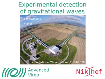
Gravitational Wave Data Analysis:

• I. Detection

Chris Van Den Broeck

Kavli RISE Summer School on Gravitational Waves, Cambridge, UK, 23-27 September 2019

Advanced LIGO and Advanced Virgo

Supernovae

Detectable astrophysical sources?

Fast-spinning neutron stars Merging neutron stars, black holes Primordial gravitational waves

Inspiral-merger-ringdown

The first detections

• Ten published binary black hole detections so far:

GW150914, GW151012, GW151226, GW170104, GW170608, GW170729, GW170809, GW170814, GW170818, GW170823

• Binary neutron star: GW170817

LIGO + Virgo, PRL 116, 061102 (2016)

Ø Einstein field equations: Ø Far away from matter/energy: Metric tensor is that of flat spacetime with a small perturbation Ø Einstein equations reduce to a wave equation for the perturbation: Ø In the “transverse-traceless” gauge, wave moving in z direction becomes:

Gravitational waves

gµν = ηµν + hµν

✓ ∂2 c2∂t2 + ∂2 ∂x2 + ∂2 ∂y2 + ∂2 ∂z2 ◆ hµν = 0

Rµ⌫ − 1 2R gµ⌫ = 8⇡G c4 Tµ⌫

Ø Consider two point particles in free fall, small separation Ø Geodesics: Ø Take the difference of the two, expand to leading order in : Ø Local Lorentz frame: Ø Non-relativistic motion: Ø Relate to the Riemann tensor: Ø In terms of the TT metric perturbation: Ø Hence tidal effect

The effect of gravitational waves on matter

Ø Gravitational waves have the effect of traveling tidal waves Ø Nearby point particles in free fall, small separation : tidal effect Ø Effect of “plus” and “cross” polarizations on ring of test particles:

Gravitational waves

h+

h×(

Ø Exploit tidal effect on matter Ø Resonant detectors § Metal bar: resonant frequency § Measure tiny length changes § Also spherical resonant detectors: equal sensitivity in all directions (e.g. miniGRAIL, Leiden)

Detection of gravitational waves

Ø Interferometric detectors § Laser beam through beam splitter § Power builds up in long (several km) cavities § At output: destructive interference … unless gravitational wave present

Interferometric detectors

Ø Motion of the end mirrors: … hence Ø Measured strain:

Interferometric detectors

x y

x y

Ø For L-shaped detectors: Ø More generally: Ø Detector tensor:

Interferometric detectors

h(t) = 1 2(hxx hyy)

Ø Signal from arbitrary direction In transverse-traceless frame: Ø If then Ø In general, need to apply linear transformation Ø Projection onto detector is also linear, hence

Interferometric detectors

h(t) = 1 2(hxx hyy)

x0 = x, y0 = y, z0 = z

x0 y0 z0

x y

x y

z

Ø Signal from an L-shaped interferometer: Ø sky position, polarization angle

Interferometric detectors

Digging a signal out of noise

Ø If there is a signal: measured strain is a sum of noise and signal: Ø If shape of signal approximately known: integrate against the output

• scillatory positive definite

period of the GW signal characteristic signal amplitude characteristic amplitude of the noise Ø To detect a signal, don’t need but only § Binary coalescences: § Millisecond pulsars:

τ0 ⇠ 102 s, T ⇠ 100 s ! (τ0/T)1/2 ⇠ 102

τ0 ⇠ 1 ms, T ⇠ 1 yr ! (τ0/T)1/2 ⇠ 105

h0 > n0

h0 > (τ0/T)1/2 n0 s(t) = n(t) + h(t)

Characterizing the noise

Ø Detector data comes in as a time series Ø If only noise: where Ø Often convenient to take a (discrete) Fourier transform: where § Notation: Ø Some noise realizations are more probable than others § Probability distribution in each frequency bin: Ø We will assume that the noise is stationary and Gaussian: Stationarity and Gaussianity: Ø Probability density for noise realization as a whole:

(n(t0), n(t1), . . . , n(tN))

ti+1 = ti + ∆t (˜ n(f0), ˜ n(f1), . . . , ˜ n(fN)) fi+1 = fi + ∆f ˜ n(fi) = ˜ ni

p(˜ ni)

p(˜ ni) / e

|˜

ni|2 2σ2 i

hnii = Z ˜ ni p(˜ ni) d˜ ni = 0, h|ni|2i = Z |˜ ni|2 p(˜ ni) d˜ ni

p[n] = p(˜ n0, ˜ n1, . . . , ˜ nN) =

N

Y

i=1

p(˜ ni)

Characterizing the noise

Ø Probability density for noise realization as a whole: Ø For stationary, Gaussian noise: Ø For the purpose of this lecture, convenient to take continuum limit: Ø Variance:

p[n] = p(˜ n0, ˜ n1, . . . , ˜ nN) =

N

Y

i=1

p(˜ ni) p[n] =

N

Y

i=1

p(˜ ni) = N e

1

2

PN

i=1 |˜ ni|2 σ2 i

p[n] = N e

1

2

PN

i=1 |˜ ni|2 σ2 i

= N e

1

2

PN

i=1 |˜ ni|2 σ2 i ∆f ∆f

! N e

R ∞

−∞ |˜ n(f)|2 Sn(f) d

f

Characterizing the noise

Ø Probability density and variance for noise realizations: Ø Could also have worked in the time domain § Stationarity: § Gaussianity: completely determined by where again denotes average over noise realizations Defining noise power spectral density as

• ne finds

p[n] = N e−

R ∞

−∞ |˜ n(f)|2 Sn(f) d

f

Characterizing the noise

Ø (Square root of ) noise power spectral density in the first two observing runs of Advanced LIGO and Advanced Virgo:

Matched filtering

Ø Instead of integrating the data against waveforms, use more optimal filter Ø Define to be the expected value of when a signal is present, and let be the root-mean-square value when no signal is present: Ø Define signal-to-noise ratio: Ø Our task: find out which filter maximizes § Do this assuming particular signal shape § Filter will be optimized for that particular signal! § Will deal later with case of many possible signal shapes S N

S N ˆ s

S N h(t)

S N S = hˆ sih N = ⇥ hˆ s2ih=0 hˆ si2

h=0

⇤1/2

S/N = hˆ sih [hˆ s2ih=0 hˆ si2

h=0]1/2

K(t)

S/N

h

ˆ s = Z ∞

−∞

dt s(t) K(t) |{z}

filter

Matched filtering

Ø Write in the frequency domain: Ø Also :

S N

S N

S = hˆ sih = Z 1

1

dt hs(t)i K(t) = Z 1

1

dt h(t) K(t) = Z 1

1

d f ˜ h(f) ˜ K⇤(f) N = ⇥ hˆ s2i hˆ si2⇤1/2

h=0

= ⇥ hˆ s2i ⇤1/2

h=0

= Z 1

1

dt Z 1

1

dt0 hn(t) n(t0)iK(t) K(t0) 1/2 = Z 1

1

d f 1 2Sn(f) | ˜ K⇤(f)|2 1/2

Matched filtering

Ø Then we arrive at: Ø Now define the noise-weighted inner product … and rewrite as … or Maximizing is equivalent to making point in the same direction as

S N = R 1

1 d

f ˜ h(f) ˜ K⇤(f) hR 1

1 d

f 1

2Sn(f) | ˜

K(f)|2 i1/2

(A|B) ⌘ < Z 1

1

d f ˜ A⇤(f) ˜ B(f)

1 2Sn(f)

= 4 < Z 1 d f ˜ A⇤(f) ˜ B(f) Sn(f) S/N

S N = (K|h) (K|K)1/2 K = 1 2Sn(f) ˜ K(f)

S N = ( ˆ K|h) ˆ K = K (K|K)1/2

S/N ˆ K h

Matched filtering

Ø Maximizing is equivalent to making point in the same direction as Ø Optimal signal-to-noise ratio

S/N ˆ K h

S N = ( ˆ K|h) ˆ K = K (K|K)1/2

ˆ K / h ! K / h

! ˜ K(f) / ˜ h(f) Sn(f) “Wiener filter” S N = (K|h) p (K|K) = (h|h) p (h|h) = p (h|h)

K = 1 2Sn(f) ˜ K(f)

Matched filtering

Ø So far we assumed that if signal present in the data, it would be of known shape: and Ø In practice we must consider many possible trial waveforms , and apply the

• ptimal filter for each of these to the data:

Ø In practice we only know the detector output , not its expectation value, so in actual signal processing we approximate

hsi = h S/N = ( ˆ K|hsi) = ( ˆ K|h)

/ hi

ˆ Ki / hi

s

✓ S N ◆

i

= ( ˆ Ki|hsi) = (Ki|hsi) p (Ki|Ki) = (hi|hsi) p (hi|hi)

✓ S N ◆

i

' (hi|s) p (hi|hi)

Matched filtering

Ø For a given trial waveform : Ø For e.g. compact binary coalescences, waveforms are characterized by source parameters Ø Lay out template banks over parameter space: points give waveforms Ø Find maximum of signal-to-noise ratio over the template bank:

¯ θ = {θ1, θ2, . . . , θN}

✓ S N ◆

i

= (hi|s) p (hi|hi) / hi

¯ θi hi = h(¯ θi)

✓ S N ◆

max

= max

i

(h(¯ θi)|s) p (h(¯ θi)|h(¯ θi))

Placement of template banks

Ø Match between nearby templates : Ø Expand in small quantities: Ø Define a metric tensor on parameter space: Ø Mismatch between neighboring templates: Place templates on parameter space such that metric distance never larger than a pre-specified mismatch, e.g. 0.03

M = (ˆ h(¯ θ)|ˆ h(¯ θ + ∆θ))

M ' (ˆ h(¯ θ)|ˆ h(¯ θ)) + ∂M ∂θi ∆θi + 1 2 ∂2M ∂θi∂θj ∆θi∆θj = 1 + 1 2 ∂2M ∂θi∂θj ∆θi∆θj

gij ≡ −1 2 ∂2M ∂θi∂θj

1 − M = gij∆θi∆θj

ˆ h(¯ θ) = h(¯ θ)/ q (h(¯ θ)|h(¯ θ))

Placement of template banks

Ø Example of placement in § Spin dimensions not shown

(m1, m2)

Characterizing S/N in the absence of signals

Ø Glitches in the instruments can pose as gravitational wave signals! Ø Given data from multiple detectors, slide data streams in time w.r.t. each other § Collect the values of S/N for all instances where the same template (same parameters) gave the highest S/N in both detector outputs § Because of the time-sliding, these won’t be astrophysical events! § Gives us the distribution of S/N for real detector noise Ø Distribution of S/N for noise triggers in Gaussian simulated noise (blue) and real data (red): § Given a candidate signal, assess its statistical significance by comparing with the red distribution

The first detection: GW150914

Ø Initial search used 16 days of two-detector data for background calculation § Significance > 5.1σ § False alarm rate < 1 in 203000 years

“Burst” sources

Ø Any transient sources

§ Supernovae in or near the galaxy § Cosmic string “cusps” or “kinks” § Long gamma-ray bursts § Soft gamma-ray repeater giant flares § Neutron star instabilities § … § The unknown

Ø Many of these are poorly modeled

§ Can’t necessarily use matched filtering

“Burst” sources

Detection without a (good) signal model Ø Look for “coherent” signals

§ Present in multiple detectors § Consistent given differences in detector responses

• “Project out” the detector noises

using a projection operator constructed from the antenna pattern functions

• Define a “likelihood” for a coherent

signal to be present; will play the role of S/N

• Construct a background distribution

to assess significance of events

The first detection: GW150914

Ø “Burst” searches also capture binary coalescences! § GW150914 seen with unmodeled search at 4.4σ

GWTC-1: Gravitational Wave Transient Catalog from first and second Advanced LIGO/Virgo science runs

FAR [y−1] Network SNR Event UTC Time PyCBC GstLAL cWB PyCBC GstLAL cWB GW150914 09:50:45.4 < 1.53 × 10−5 < 1.00 × 10−7 < 1.63 × 10−4 23.6 24.4 25.2 GW151012 09:54:43.4 0.17 7.92 × 10−3 – 9.5 10.0 – GW151226 03:38:53.6 < 1.69 × 10−5 < 1.00 × 10−7 0.02 13.1 13.1 11.9 GW170104 10:11:58.6 < 1.37 × 10−5 < 1.00 × 10−7 2.91 × 10−4 13.0 13.0 13.0 GW170608 02:01:16.5 < 3.09 × 10−4 < 1.00 × 10−7 1.44 × 10−4 15.4 14.9 14.1 GW170729 18:56:29.3 1.36 0.18 0.02 9.8 10.8 10.2 GW170809 08:28:21.8 1.45 × 10−4 < 1.00 × 10−7 – 12.2 12.4 – GW170814 10:30:43.5 < 1.25 × 10−5 < 1.00 × 10−7 < 2.08 × 10−4 16.3 15.9 17.2 GW170817 12:41:04.4 < 1.25 × 10−5 < 1.00 × 10−7 – 30.9 33.0 – GW170818 02:25:09.1 – 4.20 × 10−5 – – 11.3 – GW170823 13:13:58.5 < 3.29 × 10−5 < 1.00 × 10−7 2.14 × 10−3 11.1 11.5 10.8 LIGO + Virgo, PRX 9, 031040 (2019)

Continuous gravitational waves

Ø Emission by fast-spinning neutron stars § Isolated neutron stars: asymmetry due to “starquakes” § Neutron stars orbiting around an ordinary star: asymmetry due to accretion Ø Signals are weak: § But long-lived, can integrate for long time Ø Searches: § All-sky

• Includes stars that have not (yet) been seen

electromagnetically

§ “Directed”

• Sky position known, but not frequency

(e.g. Cas A supernova remnant)

§ “Targeted”

• Sky position and frequency known

(e.g. Crab pulsar, Vela pulsar)

Continuous gravitational waves

Searching for a sinusoid can be computationally expensive! Ø Account for Doppler modulation due to motion of the Earth:

§ Binning in sky position: up to (few)x105 points

Ø Even given a sky position, need to account for changes in frequency due to spin-down:

§ Binning in spin-down coefficients: typically O(106) points

Stochastic gravitational waves

Ø Gravitational wave backgrounds of a fundamental nature

§ Inflation: period of exponential growth of the Universe § Phase transitions: fundamental forces splitting off § Cosmic strings § …

Ø Combined background of weak signals from astrophysical sources

§ Coalescing binaries out to arbitrary distances § All the continuous waves sources in the Milky way § …

Stochastic gravitational waves

Ø Takes the form of “noise” that is correlated between detectors

§ Searched for by cross-correlating between detectors: § Optimal filter:

Ø In the case of astrophysical stochastic background from binary coalescences: Detection in a few years’ time?

Y = Z ˜ s1(f) ˜ K(f) ˜ s2(f) d f ˜ K(f) ∝ γ(f) Ωgw(f) f 3 Sn,1(f) Sn,2(f) Ωgw(f) ≡ Ω0 f α

Summary

Ø Advanced LIGO and Virgo have been detecting binary black hole and binary neutron star coalescences § Now in the regime of ~1 detection per week! Ø Wealth of gravitational wave sources: Ø Coalescing binaries composed of neutron stars or black holes Ø “Burst” events: supernovae, cosmic strings, …, the unknown? Ø Continuous waves from fast-spinning neutron stars Ø Stochastic backgrounds Ø More on the way!