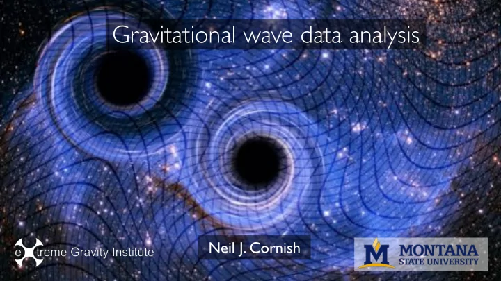
Gravitational wave data analysis Neil J. Cornish Resources - PowerPoint PPT Presentation

Gravitational wave data analysis Neil J. Cornish

Resources Papers/Reviews LIGO/Virgo, “A guide to LIGO–Virgo detector noise and extraction of transient gravitational-wave signals”, CQG 37 , 055002 (2020) https://inspirehep.net/files/b2372 ff edccfa26c93e8adbb14e6208c Cornish “Black Hole Merging and Gravitational Waves”, Black Hole Formation and Growth, Saas-Fee Advanced Course 48, (2019) https://www.dropbox.com/s/l8nusg5fd5x3ak1/2019_Book_BlackHoleFormationAndGrowth.pdf?dl=0 Books Maggiore, “Gravitational Waves: Volume 1: Theory and Experiments” Creighton & Anderson “Gravitational-Wave Physics and Astronomy: An Introduction to Theory, Experiment and Data Analysis”

Gravitational Wave Detectors - Time of Flight

Detector Response to GWs ∆ ν ( t ) = d ∆ T ( t ) ∆ T ( t ) Φ ( t ) = 2 πν 0 ∆ T ( t ) dt ν 0 t ^ ^ ^ ^ ^ v Δ T(t) ^ u beam splitter end mirror 2 end mirror 1 Pulsar Timing Spacecraft tracking Laser Interferometers

The Long and the Short of it f ∗ = c L LIGO LISA PTA

Time of flight computed in TT gauge ds 2 = − dt 2 + dx 2 (1 + h + ( u )) + dy 2 (1 − h + ( u )) + 2 h × ( u ) dydy + dz 2 dx = − dvdu + dx 2 (1 + h + ( u )) + dy 2 (1 − h + ( u )) + 2 h × ( u ) dydy dx where u = t − z, v = t + z All time-of-flight detectors require us to compute the time it takes a photon to travel from one event to another in the spacetime perturbed by a GW. Some require multiple trips t ^ ^ ^ ^ ^ v Δ T(t) ^ u beam splitter end mirror 2 end mirror 1 [See N. J. Cornish, Phys.Rev.D80:087101,2009, arXiv:0910.4372]

̂ ̂ Time of flight computed in TT gauge ∆ τ 12 = (ˆ a ⊗ ˆ a ) : H [ u 1 , u 2 ] ( u = k α x α ) 2(1 − ˆ k · ˆ a ) } δ t Here is a unit vector along the detector arm and is the GW propagation direction a k Z u 2 h = h + ( u ) ✏ + + h × ( u ) ✏ × H [ u 1 , u 2 ] = h ( u ) du ˆ a (0 , 0 , 0 , 0) u 1

General coordinate system n = sin θ cos φ ˆ x + sin θ sin φ ˆ y + cos θ ˆ ˆ z u = cos θ cos φ ˆ x + cos θ sin φ ˆ y − sin θ ˆ ˆ z v = sin φ ˆ x − cos φ ˆ ˆ y ˆ u ˆ n e + = ˆ ψ ( u ⊗ ˆ u − ˆ v ⊗ ˆ v ˆ p z e × = ˆ u ⊗ ˆ v + ˆ v ⊗ ˆ u ˆ ˆ q v ˆ h = h + � + + h × � × k � � � + = p ⊗ ˆ ˆ p − ˆ q ⊗ ˆ � q y cos 2 � e + − sin 2 � e × = � × = p ⊗ ˆ ˆ q + ˆ q ⊗ ˆ p � sin 2 � e + + cos 2 � e × = x

Example: Laser interferometer in the long wavelength limit ∆ T ( t ) = ∆ τ 12 + ∆ τ 24 − ∆ τ 13 − ∆ τ 34 t 4 ^ h ( t ) ≡ ∆ T ( t ) ≈ 1 h i a − ˆ b ⊗ ˆ a ⊗ ˆ ˆ : h ( t ) b ^ 2 L 2 3 Detector tensor ^ 2 h ( t ) = h + ( t ) ✏ + + h × ( t ) ✏ × ^ ^ v Δ T(t) ˆ b ^ ˆ u a beam splitter end mirror 2 1 Polarization tensors end mirror 1

Antenna Pattern Functions e + = ˆ u ⊗ ˆ u − ˆ v ⊗ ˆ n = sin θ cos φ ˆ x + sin θ sin φ ˆ y + cos θ ˆ ˆ v z e × = ˆ u = cos θ cos φ ˆ x + cos θ sin φ ˆ y − sin θ ˆ ˆ z u ⊗ ˆ v + ˆ v ⊗ ˆ u v = sin φ ˆ x − cos φ ˆ ˆ y ˆ u ˆ n ψ ( cos 2 θ cos 2 φ − sin 2 φ a ) : e + (ˆ a ⊗ ˆ = ˆ p z ˆ ˆ q v a ) : e × (ˆ a ⊗ ˆ = cos θ sin 2 φ ˆ k cos 2 θ sin 2 φ − cos 2 φ (ˆ b ⊗ ˆ b ) : e + = y ˆ b ˆ a (ˆ b ⊗ ˆ b ) : e × = − cos θ sin 2 φ x

Antenna Pattern Functions e + = ˆ u ⊗ ˆ u − ˆ v ⊗ ˆ n = sin θ cos φ ˆ x + sin θ sin φ ˆ y + cos θ ˆ ˆ v z e × = ˆ u = cos θ cos φ ˆ x + cos θ sin φ ˆ y − sin θ ˆ ˆ z u ⊗ ˆ v + ˆ v ⊗ ˆ u v = sin φ ˆ x − cos φ ˆ ˆ y ˆ u ˆ n h = F + h + + F × h × ψ ( ˆ p z ˆ ˆ q v 1 a − ˆ b ⊗ ˆ F + b ) : � + = 2(ˆ a ⊗ ˆ ˆ k 1 2(1 + cos 2 � ) cos(2 � ) cos 2 � − cos � sin 2 � sin 2 � = 1 a − ˆ b ⊗ ˆ y F × b ) : � × = 2(ˆ a ⊗ ˆ ˆ b ˆ a 1 2(1 + cos 2 � ) cos(2 � ) sin 2 � + cos � sin 2 � cos 2 � = x

Antenna Pattern Functions q F 2 + + F 2 F + F × F = × Polarization averaged

Terrestrial Network H H V K L I L K I V

Terrestrial Network H H V K L I L K I V

Terrestrial Network H H V K L I L K I V

Terrestrial Network H H V K L I L K I V

Terrestrial Network H H V K L I L K I V

Terrestrial Network H H V K L I L K I V

Laser Interferometer Space Antenna Low frequency response

Beyond the low frequency approximation Z u 2 ∆ τ 12 = (ˆ a ⊗ ˆ a ) : H [ u 1 , u 2 ] ( u = k α x α ) H [ u 1 , u 2 ] = h ( u ) du 2(1 − ˆ k · ˆ a ) u 1 h ( u ) = A cos( ω ( t − ˆ k · x )) ✏ + Example: " # ˆ  ω L � k · ( x 1 + x 2 ) ∆ τ 12 = L ω ( t + L 2 (1 − ˆ a ) : ✏ + ) sinc 2 ((ˆ a ⊗ ˆ k · ˆ a ) cos 2 − 2 Finite arm-length Long wavelength one- Phase of the wave correction to arm antenna pattern at midpoint of arm antenna pattern

Pulsar Timing (note that here the photons − ˆ propagate in the direction) a � 0 τ GW ( t ) = − L (ˆ a ⊗ ˆ a ) : h ( t + L ξ , − ˆ a ξ L ) d ξ n − ξ L ˆ k = − ˆ D (ˆ a − ˆ n cos µ ) 2 − 1 { GW ˆ k D ˆ n L ˆ a fL = 10 , ψ = 0 µ (ˆ a ⊗ ˆ a ) : H = (1 + cos µ )( H + cos 2 ψ + H × sin 2 Ψ ) (Ignoring L/D amplitude corrections)

Data Analysis 101 - Laplace & Gauss Pierre Simon de Laplace Carl Friedrich Gauss Memoir on the Probability of Causes of Events (1774) Analytical Theory of Probability (1812) ︎ Z. Astronom. Verwandte Wiss. 1 185, (1816) Laplace developed Bayesian Inference. Gauss developed maximum likelihood estimation. Gauss introduced the normal distribution, Laplace explained its ubiquity (CLT). 4 4 model data 3 3 2 2 1 1 0 d 0 d -1 -1 -2 -2 -3 -3 -4 -4 0 0.2 0.4 0.6 0.8 1 0 0.2 0.4 0.6 0.8 1 x x

Data Analysis 101 4 4 data model 3 3 2 2 1 1 0 0 d d — -1 -1 -2 -2 -3 -3 -4 -4 0 0.2 0.4 0.6 0.8 1 0 0.2 0.4 0.6 0.8 1 x x 4 residual = data - model 3 2 1 = 0 d -1 -2 -3 -4 0 0.2 0.4 0.6 0.8 1 x

Data Analysis 101 ⇒ d = h + n d − h = n 4 The residuals should follow the noise distribution residual = data - model 3 In this example the noise was uncorrelated between samples and 2 draw from a Gaussian distribution with a fixed standard deviation (“stationary white noise”) 1 0 d − n 2 i -1 1 2 σ 2 p ( n i ) = e -2 2 πσ -3 N n 2 ∑ i -4 − p ( n ) = ∏ 1 2 σ 2 0 0.2 0.4 0.6 0.8 1 p ( n i ) = (2 π ) N /2 σ N e i =1 x i

Data Analysis 101 4 4 data residual = data - model model 3 3 2 2 1 1 0 0 d d -1 -1 -2 -2 -3 -3 -4 -4 0 0.2 0.4 0.6 0.8 1 0 0.2 0.4 0.6 0.8 1 x x The likelihood of observing the data d given the model h is simply N ( d i − h i ) 2 ∑ − 1 2 σ 2 p ( d − h ) = (2 π ) N /2 σ N e i =1

Data Analysis 101 If the noise is correlated between data samples (“colored noise”), and/or if the amplitude of the noise changes from sample to sample (“heteroskedastic” aka “non-stationary”), then we need to generalize the Gaussian likelihood: 2 ( d i − h i ) C − 1 1 ij ( d j − h j ) (det(2 π C )) N /2 e − 1 p ( d − h ) = In the previous example the noise correlation matrix was promotional to the identity matrix: C SWN = δ ij σ 2 ij The quantity in the exponent is the chi squared goodness of fit χ 2 = ( d i − h i ) C − 1 ij ( d j − h j ) ≡ ( d − h | d − h ) Here I have introduced the noise weighted inner product ( a | b ) = a i C − 1 ij b j

Data Analysis 101 Gravitational wave data comes in the form of a time series. Computing the noise-weighted inner product in the time domain is costly since the matrix is not diagonal. If the noise is stationary, i.e. has statistical properties that are unchain with time, then the noise correlation matrix is diagonal in the frequency domain. That is why most GW analysis is done in the frequency domain. a ( f )˜ a *( f )˜ ˜ b *( f ) + ˜ b ( f ) ij b j = 2 ∑ ( a | b ) = a i C − 1 S n ( f ) f The factor of 2 is because we only sum over positive frequencies. The quantity is the one-sided noise spectral density (PSD) S n ( f ) a W ( f ) = ˜ a ( f )/ S n ( f ) 1/2 We often talk about “whitened” data or waveforms. This is simply . Can transform this back to the time domain: ˜ data - signal = noise

Challenges for Gravitational Wave Data Analysis Complicated waveforms, as many as 17 parameters Noise properties have to be estimated along with the signals Non-Gaussian noise transients have to be modeled/mitigated

Challenges for Gravitational Wave Data Analysis Complicated waveforms, as many as 17 parameters Noise properties have to be estimated along with the signals Non-Gaussian noise transients have to be modeled/mitigated

The Bayesian Way Likelihood Prior (noise model) (signal model) Posterior p ( h | d ) = p ( d | h ) p ( h ) probability for p ( d ) waveform h Normalization - model evidence

Gravitational wave signal types Well modeled - e.g. binary inspiral and merger p ( h ) Poorly modeled - e.g. core collapse supernovae Stochastic- e.g. phase transition in early universe