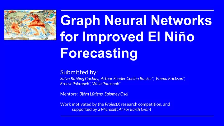
Graph Neural Networks for Improved El Nio Forecasting Submitted - PowerPoint PPT Presentation

Graph Neural Networks for Improved El Niño Forecasting Submitted by: Salva Rühling Cachay, Arthur Fender Coelho Bucker*, Emma Erickson*, Ernest Pokropek*, Willa Potosnak* Mentors: Björn Lütjens, Salomey Osei Work motivated by the ProjectX research competition, and supported by a Microsoft AI For Earth Grant

El Niño–Southern Oscillation (ENSO) ● El Niño is the warm phase the ENSO climate pattern where the cold phase is referred to as La Niña ● An irregular climate phenomenon that occurs every 2-7 years ● Causes disasters worldwide ● Affects agriculture and public health 2 Image from: https://www.climate.gov/news-features/understanding-climate/2015-state-climate-el-ni%C3%B1o-came-saw-and-conquered

Previous Research Previous Machine Learning (ML) for El Niño/Southern Oscillation (ENSO) r esearch showed improved forecasting with the use of Convolutional Neural Networks (CNNs). This method outperformed state-of-the-art dynamical models by using sea surface temperature (SST) and heat content anomalies as model input. The predictand was the Oceanic Niño Index (ONI), a common measure of ENSO. 3 Y.-G. Ham, J.-H. Kim, and J.-J. Luo, “Deep learning for multi-year enso forecasts,” Nature, vol. 573, pp. 568–572, 9 2019

Motivation Long-term ENSO forecasts have remained at low skill due to: 1. The high variability in ENSO manifestations 2. The complexity of its teleconnections, i.e. interlinked, large-scale phenomena Why Graph Neural Networks (GNN)? ● The large-scale dependencies that describe climate can be modeled as graph of a GNN ● GNNs generalize the notion of locality allowing for complex, non-Euclidean connections to be modeled via edges ● Enhanced interpretability (Inductive bias) via learned (pre-defined) edges ● GNNs can overcome statistical model limitations of single-valued index output (e.g. only the coarse ONI) by forecasting target variables (SST anomalies) at target geographical regions (e.g. each node within the ONI region) 4

Project Model: Our Approach 1. Grid cells in climate dataset are individually represented as nodes V i and each corresponds to a geographical location in terms of longitude and latitude 2. These locations are mapped as nodes in the graph: G = (V, E) 3. Each node is associated with a feature vector of climate variables for each time step t 4. Edges between nodes encode information flow and inductive bias. a. Can be learnt jointly with the model’s parameters b. Selected based on domain knowledge 5

Project Model: Our Approach (cont.) 1. For our experiments, we build upon the spatiotemporal GNN proposed by Wu et al. [2] 2. We do not pre-define any edges 3. Once trained, our model can be used to project target climate variables at all nodes within the ONI region ( Experiment 1) , or to project the ONI index ( Experiment 2) , for a specified number of months in advance ONI index region 6 6 [2] Z. Wu, S. Pan, G. Long, J. Jiang, X. Chang, and C. Zhang, “Connecting the dots: Multivariate time series forecasting with graph neural networks,” KDD 2020

Enhanced Interpretability: Our GNN Learns Meaningful Connections The summed weights of incoming edges are plotted for each node . Nodes with darker colors have a central role in the graph, as the model assigns higher importance to them. Nodes with the highest importance can be seen in or near the ONI region for 1 lead month, while closely resembling the ENSO pattern for 6 lead months in terms of higher SST in the Central and Eastern Tropical Pacific*. 1 Lead Month 6 Lead Months 7 * Sea Surface Temperature Anomaly Animation of 6mon before 2015/16 El Nino (columbia.edu)

Project Overview: Data Two datasets are incorporated in this research for two separate experiments: ● Experiment 1 : SST anomalies computed from the NOAA ERSSTv5 dataset for training, validating and testing model, split in a sequential manner. We test on 1984-2020. ○ Only 1233 training samples ● Experiment 2 : We use the exact same data and data split as [1], i.e. CMIP5 simulations, and the SODA dataset with SST anomaly data for (pre-) training and GODAS dataset for testing (1984-2017). 1871 1973 1984 2020 Training Set Validation Set Test Set Exp. 1: ERSSTv5 Exp. 1: ERSSTv5 Exp. 1: ERSSTv5 Exp. 2: SODA Exp. 2: GODAS Exp. 2: CMIP5 + SODA Data as in [1] 8 8 [1] **Y.-G. Ham, J.-H. Kim, and J.-J. Luo, “Deep learning for multi-year enso forecasts,” Nature, vol. 573, pp. 568–572, 9 2019

Our Results ● Our simple, very efficient GNN1 model gives fairly skillful forecasts of the ONI as well as the zonal SSTAs (Table 1) ● Our GNN2 models outperforms the state-of-the-art CNN [1] for 1 and 3 lead months (Table 2) (but does not yet use heat content, nor additional inductive bias via pre-defined edges). ● The use of simulation data (GNN2) from a larger region of the world significantly improves model performance (Table 1). Table 1: Table 2: Correlation skill and RMSE for n lead months on ERSSTv5 Predictive correlation skill for n lead months on GODAS Metric Model n = 1 n = 3 n = 6 Model n = 1 n = 3 n = 6 n = 12 Correlation GNN1 0.9867 0.8936 0.6776 CNN [1] ca. 0.94 0.8761 0.7616 0.6515 GNN2 0.9882 0.9273 0.7755 GNN2 (ours) 0.9747 0.8908 0.7420 0.5547 RMSE GNN1 0.1278 0.3556 0.6034 GNN2 0.1202 0.2900 0.4923 9 [1] **Y.-G. Ham, J.-H. Kim, and J.-J. Luo, “Deep learning for multi-year enso forecasts,” Nature, vol. 573, pp. 568–572, 9 2019

3 Lead Month Forecast of GNN1 SST anomalies of past 12-month period were used as model input to forecast ENSO for 3-month ahead. Results show improved performance over previous CNN model with ONI forecast correlation = 0.8936 and a root-mean-square error (RMSE)= 0.356. ONI region Test period forecasts Latitude: 5°S to 5°N ERSSTv5 ONI index = Orange Longitude: 120°W to 170°W 10 GNN forecasted ONI index = Blue

GNN1 Forecasts are Independent of the Seasonal Cycle We extracted information of both the seasonal cycle and ENSO events from a single recording of the SSTAs using principal component analysis. This allowed us to determine the presence of the seasonal cycle in the used dataset computed from ERSSTv5. The heat maps indicate that the seasonal cycle is not present in this dataset, so our GNN1 model does not rely on seasonal cycle when making forecasts. 11

Exciting Future Research Directions: We plan to: Remove the potential influence of the seasonal cycle for data used in the GNN2 model ● Include additional features such as heat content anomalies ● Explore ways to potentially increase our models skill in estimating extreme ENSO events ● (e.g. via a custom loss function) Use the edge weight analysis to assess the reliability of our model and potentially look for ● yet undiscovered ENSO teleconnections Incorporate climatologists’ knowledge on known teleconnections and regions correlated ● with ENSO conditions for pre-assigning edge weights 12