GNR607 Principles of Satellite Image Processing Instructor: Prof. - - PowerPoint PPT Presentation

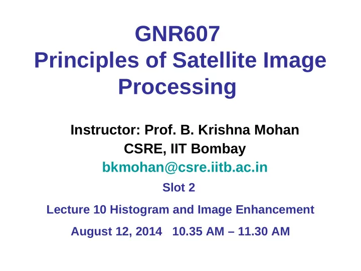
GNR607 Principles of Satellite Image Processing

Instructor: Prof. B. Krishna Mohan CSRE, IIT Bombay bkmohan@csre.iitb.ac.in

Slot 2 Lecture 10 Histogram and Image Enhancement August 12, 2014 10.35 AM – 11.30 AM

Contents of the Lecture

• Histogram of an Image
• Useful information from Histogram
• Contrast in Satellite Image

– Linear Contrast Enhancement IIT Bombay Slide 1 GNR607 Lecture 10 B. Krishna Mohan August 12, 2014 Lecture 10 Histogram and Image Enhancement

Shift Variant Systems

g(x) =

• The response of some image processing
• perators is shift variant, i.e., the form of the
• peration varies with position in the image
• e.g., A projection system that is not working well

will illuminate one part of the screen brightly while another part will be dull

GNR607 Lecture 10 B. Krishna Mohan IIT Bombay Slide 2

( ) ( , ) f h x d α α α

∫

Convolution

• For a linear shift invariant system, we can

write

• g(x) =
• This is known as the convolution integral
• For a linear shift invariant system the output
• f the system is obtained by the convolution
• f the input and the impulse response of the

system

( ) ( ) f h x d α α α

∞ −∞

−

∫

GNR607 Lecture 10 B. Krishna Mohan IIT Bombay Slide 3

Convolution

• Convolution operation is compactly represented

as g(x) = f(x) * h(x)

• f(x) * h(x) ≜

( ) ( ) f h x d α α α

∞ −∞

−

∫

GNR607 Lecture 10 B. Krishna Mohan IIT Bombay Slide 4

In discrete case,

( ) ( )* ( ) ( ) ( )

k

g n f n h n f n k h k = = −

∑

Convolution

( ) ( ) ( ) ( ) f x g x f t g x t dt

∞ −∞

∗ = −

∫

f(x) f(x) g(x) g(x)

IIT Bombay Slide 5 GNR607 Lecture 10 B. Krishna Mohan

Relevance of Linearity

• Many image processing operations are

linear

• Linear operations are easier to analyze
• They are often less time consuming to

compute

• Linear shift invariant operations can be

efficiently performed using Fourier transforms (to be discussed later)

GNR607 Lecture 10 B. Krishna Mohan IIT Bombay Slide 6

Non-linearity

• Certain processes in image acquisition are

inherently non-linear

• For example, the deposition of silver on a

photographic film in response to the amount of light incident is logarithmically related

• Our perception of brightness in relation to

the amount of incident light on the retina is also non-linear

GNR607 Lecture 10 B. Krishna Mohan IIT Bombay Slide 7

Histogram and Its Role in Image Processing

Concept of Histogram

• Given a digital image Fm,n of size MxN, we can define

f(j) = #{Fm,n = j, 0 ≤ m ≤ M-1; 0 ≤ n ≤ N-1}

• We refer to the sequence f(j), 0 ≤ j ≤ K-1, where K is the

number of gray levels in the image, as the histogram of the image.

• f(n) is interpreted as the number of times gray level n

has occurred in the image.

• Obviously,

Σn f(n) = M . N IIT Bombay Slide 8 GNR607 Lecture 10 B. Krishna Mohan

IIT Bombay Slide 9 GNR607 Lecture 10 B. Krishna Mohan

Sample Histogram

Histogram

• With digital images, we have a range of values

that can be found at a given pixel. Depending on the resolution of the sensor from which the image is acquired, the gray level values may be [0-255], [0-1023], [0-2047], [0-63], [0-127] etc. in each band

IIT Bombay Slide 10 GNR607 Lecture 10 B. Krishna Mohan

Histogram

• The normalized version of f(n) may be defined as

p(n) = f(n) / (M.N) – p(n)  probability of the occurrence of gray level n in the image (in relative freq. sense) Σn p(n) = 1 MIN = minn {f(n) | f(n) ≠0} MAX = maxn {f(n) | f(n) ≠0}

IIT Bombay Slide 11 GNR607 Lecture 10 B. Krishna Mohan

Application of Histogram

• Dynamic range of display system – min

to max range of intensities that can be displayed

• Normal range is 0 – 255 for gray scale; for

color it is 0 – 255 for red, green and blue

• If Min-Max range of data is comparable to

dynamic range of display device, good quality display is possible

IIT Bombay Slide 12 GNR607 Lecture 10 B. Krishna Mohan

IIT Bombay Slide 13 GNR607 Lecture 10 B. Krishna Mohan

Histogram of image with good contrast

Image

IIT Bombay Slide 14 GNR607 Lecture 10 B. Krishna Mohan

Histogram of Low Contrast Image

IIT Bombay Slide 15 GNR607 Lecture 10 B. Krishna Mohan

Low Contrast Image

IIT Bombay Slide 16 GNR607 Lecture 10 B. Krishna Mohan

Good Contrast Image

IIT Bombay Slide 17 GNR607 Lecture 10 B. Krishna Mohan

Good Contrast Image

IIT Bombay Slide 18 GNR607 Lecture 10 B. Krishna Mohan

Information from Histogram

• The information conveyed by the occurrence of an

event whose probability of occurrence is p(n) is given by I(n) = ln{1/p(n)} = -ln{p(n)}

• This implies that if the probability of occurrence of an

event is low, then its occurrence conveys significant amount of information

• If the probability of an event is high, the information

conveyed by its occurrence is low IIT Bombay Slide 19 GNR607 Lecture 10 B. Krishna Mohan

Average Information – Entropy

• Average information conveyed by a set of events with

probabilities p(i), i=1,2,…, is given by

• H is called entropy and is extensively used in image

processing operations

• H is highest when all probabilities are equally likely.

Hmax = -Σ n k.ln(k), where p(n) = k for all n

• H is zero when p(j)=1 for some j, and p(k) = 0 for all

k ≠ j

H = - Σn p(n) log {p(n)}

IIT Bombay Slide 20 GNR607 Lecture 10 B. Krishna Mohan

Role of Entropy

• Indicator whether very few gray levels are

actually present, or wide range of levels in sufficient numbers.

• Entropy is also used for threshold selection
• e.g., separating image into object of interest and

background

IIT Bombay Slide 21 GNR607 Lecture 10 B. Krishna Mohan

Applications of histogram

• Can be related to the discrete probability density

function

• The gray level corresponding to the highest

frequency of occurrence is called the modal level, as seen in the histogram

• If the image has two classes, the histogram may

be bimodal with means µ1 and µ2 and standard deviations σ1 and σ2 respectively.

GNR607 Lecture 10 B. Krishna Mohan IIT Bombay Slide 22

Applications of Histogram

• A threshold or cutoff T between µ1 and µ2
• All gray levels below T – one class
• Gray levels T and above – second class
• Finding the value of T - Threshold

selection.

• Indicate the classes by 0 and 255 when

displayed on the screen.

IIT Bombay Slide 23 GNR607 Lecture 10 B. Krishna Mohan

A Bimodal Histogram

Peak 1 Peak 2 Mode 1 Mode 2 n f(n) =µ 1 =µ 2 Width equal to σ

IIT Bombay Slide 24 GNR607 Lecture 10 B. Krishna Mohan

Image Statistics from Histogram

• MIN gray level MIN = n: minn f(n) ≠0
• Max gray level MAX = n: maxn f(n) ≠0
• Mean gray level

µ = Σnn.f(n) / (M.N)

• Variance

σ2 = Σnf(n)[n-µ]2 / (M.N)

• Median

Med = k: Σk

n=0 f(n) = (M.N)/2

IIT Bombay Slide 25 GNR607 Lecture 10 B. Krishna Mohan

Image Statistics from Histogram

• Skewness

Skewness is positive if the histogram is skewed to the left of the mean, i.e., it has a long tail towards the higher gray levels Skewness is negative if the histogram is skewed to the right of the mean

GNR607 Lecture 10 B. Krishna Mohan IIT Bombay Slide 26

3 3

1 ( ) ( ) ( 1) Sk n f n MN µ σ = − −

∑

Negatively skewed Positively skewed histogram histogram

Skewness

IIT Bombay Slide 27 GNR607 Lecture 10 B. Krishna Mohan n n f(n) f(n)

Image Statistics from Histogram

• Kurtosis
• For Gaussian distributions, Kurtosis = 3.

Therefore the excess kurtosis is defined by subtracting 3 from the above equation. Positive kurtosis in this case indicates a sharply peaked distribution, and negative kurtosis denotes a flat distribution, with uniform distribution being the limiting case.

GNR607 Lecture 10 B. Krishna Mohan IIT Bombay Slide 28

4 4

1 ( ) ( ) 3 ( 1) Ku n f n MN µ σ = − − −

∑

Digital Image Enhancement

Motivation for Image Enhancement

• Image data when received in its original

form often has poor visible appearance, lacking in adequate contrast to perceive the important features in it

• The visual appearance needs to be

enhanced through image enhancement procedures

IIT Bombay Slide 29 GNR607 Lecture 10 B. Krishna Mohan

E x a m p l e

IIT Bombay Slide 30 GNR607 Lecture 10 B. Krishna Mohan

What is Contrast?

• Contrast is the difference in the intensity of the
• bject of interest compared to the background

(rest of the image)

• The perceptual contrast does not change linearly

with the difference in the intensity

• The perceptual contrast is a function of the

logarithm of the difference in the object and background intensities

• This means that in the darker regions, small

changes in intensity can be noticed, but in brighter regions, the difference has to be much more

IIT Bombay Slide 31 GNR607 Lecture 10 B. Krishna Mohan

Case1

IIT Bombay Slide 32 GNR607 Lecture 10 B. Krishna Mohan

Case 2

IIT Bombay Slide 33 GNR607 Lecture 10 B. Krishna Mohan

Histogram for Image Enhancement

• Given a 1-D histogram (computed for a

black/white image or for one band in a multispectral image), it conveys information about the quality of the image.

• Positively skewed histogram – darkish

image

• Negatively skewed histogram – lightish

image

IIT Bombay Slide 34 GNR607 Lecture 10 B. Krishna Mohan

Negatively skewed Positively skewed histogram histogram IIT Bombay Slide 35 GNR607 Lecture 10 B. Krishna Mohan

Information from Histogram

• Minimum and maximum gray levels in the

image

• Imin = min {i | h(i) ≠ 0}
• Imax = max {i | h(i) ≠ 0}
• A poor contrast image will have (Imax – Imin)

range much less than the display range of the monitor or printer.

IIT Bombay Slide 36 GNR607 Lecture 10 B. Krishna Mohan

Low Contrast Image

IIT Bombay Slide 37 GNR607 Lecture 10 B. Krishna Mohan

Image Histogram

IIT Bombay Slide 38 GNR607 Lecture 10 B. Krishna Mohan

Quality of Image Display

• Separation between minimum and

maximum levels in the image should match the dynamic range of the display system

• High Imin or small Imax will result in poor visual

quality images due to lack of contrast – difference in brightness of object of interest relative to background

IIT Bombay Slide 39 GNR607 Lecture 10 B. Krishna Mohan

Adjustment of Contrast

• This is done in several ways

– Linearly, from minimum to maximum level – Preferential adjustment, emphasis on dark levels – Preferential adjustment, emphasis on bright levels – Preferential adjustment, emphasis on number

• f pixels at each gray level

– Based on a desired histogram shape

IIT Bombay Slide 40 GNR607 Lecture 10 B. Krishna Mohan

Global Operations on Images

• Global operations are applied to the pixels

in the image, without taking note of their locations.

• g = H(f) where H is some operation on the

image f.

• If location of the pixel is also included,

then it is a local operation

IIT Bombay Slide 41 GNR607 Lecture 10 B. Krishna Mohan

Point Operations

• Point Operations are applied to pixels

solely on the basis of the gray levels found there, without taking into account the pixel position.

• Point operations lead to mapping of gray

levels from one set of values to another set.

• gij = Q[fij], where Q is some transformation

IIT Bombay Slide 42 GNR607 Lecture 10 B. Krishna Mohan

Point Operations

• In case of point operations, gray level transformations

need NOT be computed at each pixel in the image

• If the number of bits assigned to each pixel is L, then the

transformation has to be computed only for 2L gray values, 0 , 1, … , 2L-1

• This permits creating a look-up table for mapping each

gray level to its new level, supported by display hardware and facilitated by programming libraries IIT Bombay Slide 43 GNR607 Lecture 10 B. Krishna Mohan

f1 f2 f3 f4 … fn g1 g2 g3 g4 … gn Input Output

Linear Contrast Stretch

• Suppose the display range of the monitor

is ymin to ymax, which means the monitor can display (ymax – ymin + 1) levels

• Example: ymin = 0

ymax = 255

• Let the input range in the dat be xmin to xmax.

IIT Bombay Slide 44 GNR607 Lecture 10 B. Krishna Mohan

Linear Contrast Stretch

• When the input image has poor contrast, then

the range of gray levels in the image is much less than the display range of the monitor

• (ymax – ymin) >> (xmax – xmin)
• If xmax is in the left half of the gray scale, then the

image appears dark

• If xmin appears in the right half of the gray scale,

then the image appears light or faded out

IIT Bombay Slide 45 GNR607 Lecture 10 B. Krishna Mohan

Un-enhanced image in ERDAS

• After loading the image into the viewer,

select

• Raster – Contrast – General Contrast –

Linear – (Gain=1.0 and Offset=0)

• This step removes any default contrast

enhancement performed by ERDAS and displays the image as it originally is.

IIT Bombay Slide 46 GNR607 Lecture 10 B. Krishna Mohan

Linear Contrast Stretch

• Low contrast images can be linearly enhanced

using simple contrast stretch operations. Then the linear contrast stretch operation is defined by

max min min min max min min max min max min

( ) = m.( ), where y y y y x x x x x x y y m x x − − = − − − − = − x is the input level and y is the output level

IIT Bombay Slide 47 GNR607 Lecture 10 B. Krishna Mohan

ymax ymin xmin xmax Input level

Linear Contrast Stretch

m > 1  stretching m < 1  compressing m is the slope of the line Output level m=1 line IIT Bombay Slide 48 GNR607 Lecture 10 B. Krishna Mohan

Low Contrast Image

IIT Bombay Slide 49 GNR607 Lecture 10 B. Krishna Mohan

After linear contrast stretch

IIT Bombay Slide 50 GNR607 Lecture 10 B. Krishna Mohan

Low Contrast Image

IIT Bombay Slide 51 GNR607 Lecture 10 B. Krishna Mohan

After Enhancement

IIT Bombay Slide 52 GNR607 Lecture 10 B. Krishna Mohan

Contd…