GLAD: Learning Sparse Graph Recovery Le Song Georgia Tech Joint - PowerPoint PPT Presentation

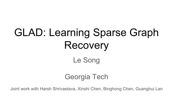
GLAD: Learning Sparse Graph Recovery Le Song Georgia Tech Joint work with Harsh Shrivastava, Xinshi Chen, Binghong Chen, Guanghui Lan

Objective Recovering sparse conditional independence graph G from data Θ "# = 0 ⇔ 𝑌 " ⊥ 𝑌 # | 𝑝𝑢ℎ𝑓𝑠 𝑤𝑏𝑠𝑗𝑏𝑐𝑚𝑓𝑡 Θ

Applications Biology Finance

Convex Formulation ● Given M samples from a distribution: ● Estimate the matrix ‘ϴ’ corresponding to the sparse graph Objective function: L1 regularized log-determinant estimation Covariance matrix Regularization 𝛵 = 𝑌 7 𝑌 Parameter 5 𝑁

Existing Optimization Algorithms G-ISTA Proximal gradient method

Existing Optimization Algorithms Glasso G-ISTA Block Proximal coordinate gradient descent method method Updates each column (and the corresponding row) of the precision matrix iteratively by solving a sequence of lasso problems

Existing Optimization Algorithms ADMM Glasso G-ISTA Alternating Block Proximal direction coordinate gradient method of descent method multipliers method

Hard to Tune Hyperparameters ‘Grid search’ is tedious and non-trivial Tuning hyperparameters for Traditional Methods Errors of different Outcomes highly sensitive parameter combinations to penalty parameters

Mismatch in Objectives mismatch! Recovery Log-determinant Objective estimator (NMSE) / Θ ∗ < ;

Limitations of Existing Optimization Algorithms Based on ‘carefully chosen conditions’ like Consistency of 1. Lower bound on sample size estimator 2. Sparsity of Ө 3. Degree of graph 4. Magnitude of covariance entries Limitations of the Room for convex formulation Improvement! Specific 1. Highly sensitive parameter regularization 2. Depends on tail behavior of maximum parameter deviation Pradeep Ravikumar, Martin J Wainwright, Garvesh Raskutti, Bin Yu, et al. High-dimensional covariance estimation by minimizing l1-penalized log-determinant divergence. Electronic Journal of Statistics, 5:935–980, 2011.

Big Picture Question Given a collection of ground truth precision matrix Θ ∗ , and the corresponding ● empirical covariance 5 Σ Learn an algorithm 𝑔 which directly produces an estimate of the precision ● matrix Θ ? 1 < , 𝑡. 𝑢. Θ " = 𝑔( F ∗ min E Θ " − Θ " Σ " ) ; |𝒠| B ∗ ∈𝒠 F G H ,J H

Deep Learning Model Example DeepGraph (DG) ` architecture.The input is first standardized and then the sample covariance matrix is estimated. A neural network consisting of multiple dilated convolutions (Yu & Koltun, 2015) and a final 1 × 1 convolution layer is used to predict edges corresponding to non-zero entries in the precision matrix. * DeepGraph-39 model from Fig.2 of “Learning to Discover Sparse Graphical Models” by Belilovsky et. al.

Challenges in Designing Learning Models Traditional Approaches #parameters #parameters scale dim^2 scale 𝐸×𝐸 DNNs DNNs Permutation Permutation SPD SPD CNNs CNNs Challenges Challenges Invariance Invariance constraint constraint Autoencoders, Autoencoders, VAEs, RNNs VAEs, RNNs Interpretable Interpretable

GLAD: DL model based on Unrolled Algorithm Alternating Minimization (AM) algorithm: Objective function AM: Update Equations (Nice closed form updates!) ● Unroll to fixed #iterations ‘K’. ● Treat it as a deep model

GLAD: Training Loss function: Frobenius norm with discounted cumulative reward Gradient Computation through matrix square root in the GLADcell: For any SPD matrix X: Solve Sylvester’s equation for d ( X 1/2 ): Optimizer for training: ‘Adam’. Learning rate chosen between [0.01, 0.1] in conjunction with Multi-step LR scheduler.

Use Neural Networks for ( ⍴ , λ) ↕ ( ⍴ NN , λ NN ) # of layers # of layers Minimalist = 2 = 4 designing of Neural Hidden unit Hidden unit Networks size = 3 size = 3 Non-Linearity: Hidden layers = ‘ tanh ’ Final layer = ‘ sigmoid ’

GLAD GLAD Using algorithm GLADcell structure as inductive bias for designing unrolled DL architectures

Desiderata for GLAD Minimalist Minimalist Model Model Permutation Permutation SPD SPD GLAD GLAD Invariance Invariance constraint constraint Interpretable Interpretable GLAD: G raph recovery L earning A lgorithm using D ata-driven training

Experiments: Convergence Train/finetuning using 10 random graphs Fixed Sparsity level Test on 100 s=0.1 random graphs GLAD vs traditional methods Mixed Sparsity level s 〜 U(0.05, 0.15)

Experiments: Recovery probability Sample complexity for model selection consistency PS is non-zero if all graph edges are recovered with correct signs GLAD able to recover true edges with considerably fewer samples

Experiments: Data Efficiency (cont...) Methods M=15 M=35 M=100 GLAD vs CNN* BCD 0.578±0.006 0.639±0.007 0.704±0.006 Training graphs CNN 0.664±0.008 0.738±0.006 0.759±0.006 100 vs 100,000 CNN+P 0.672±0.008 0.740±0.007 0.771±0.006 # of parameters <25 vs >>>25 GLAD 0.788±0.003 0.811±0.003 0.878±0.003 Runtime < 30 mins vs AUC ` on 100 test graphs, Gaussian random graph sparsity=0.05 several hours and edge values sampled from ~U(-1, 1). * DeepGraph-39 model from “Learning to Discover Sparse Graphical Models” by Belilovsky et. al. ` Table 1. of Belilovsky et. al.

Gene Regulation Data: SynTReN details Synthetic gene expression Models biological & data generator creating correlation noises biologically plausible networks SynTReN The topological characteristics Contains instances of Ecoli of generated networks closely bacteria and other true resemble transcriptional interaction networks networks

Gene Regulation Data: Ecoli Network Predictions GLAD trained on Erdos-Renyi graphs of dimension=25. # of train/valid graphs were 20/20. M samples were generated per graph Recovered graph structures for a sub-network of the E. coli consisting of 43 genes and 30 interactions with increasing samples. All noises sampled ~U(0.01, 0.1) Increasing the samples reduces the fdr by discovering more true edges.

Theoretical Analysis: Assumptions Ensures that sample sizes are large enough for an accurate estimation of the covariance matrix Restricts the interaction between edge and non-edge terms in the precision matrix

Consistency Analysis Recalling AM Update Equations An adaptive sequence of penalty parameters should achieve a better error bound Optimal parameter values Summary depends on the tail behavior and the prediction error Hard to choose these parameters manually

Conclusion Unrolled DL architecture, Empirically, GLAD is able to GLAD, for sparse graph reduce sample complexity recovery Highlighting the potential of Empirical evidence that using algorithms as learning can improve inductive bias for DL graph recovery architectures

Thank you!