Get a handout 1 Welcome to DS504/CS586: Big Data Analytics - PowerPoint PPT Presentation
Get a handout 1 Welcome to DS504/CS586: Big Data Analytics --Review Prof. Yanhua Li Time: 6:00pm 8:50pm R Location: AK233 Spring 2018 Next Session: Final Project Presentation v 12/24 T: Submission day Project reports to discussion
Get a handout 1
Welcome to DS504/CS586: Big Data Analytics --Review Prof. Yanhua Li Time: 6:00pm –8:50pm R Location: AK233 Spring 2018
Next Session: Final Project Presentation v 12/24 T: Submission day Project reports to discussion board v Self-&-cross evaluation form to Assignment v v 12/26 R: Presentation Day Quiz 2 (I will send you sample questions soon) v v 20 min each team (including Q&A) v Team 1 v Team 2 v 10 min break v Team 3 v Team 4 v Team 5 3 v Snacks and soft drink will be provided.
Today • 1. CityLines • 2. Review – Key topics, techniques, discussed in the semester – Future opportunities • Big data analytics • Urban Computing – 10 min break 7:20-7:30PM • 2. Team 5 presentation and discussion: 7:30-8:30PM • 3. Course evaluation 8:30PM-8:45PM • 4. Finish at 8:45PM – (last week we finished 5 minutes late.)
CityLines: Hybrid Hub-and-Spoke System for Urban Transportation Services Yanhua Li Assistant Professor Computer Science Department Worcester Polytechnic Institute
Global Urbanization and Transportation
Today’s Urban Transit Services Public Transits Private Transit affordable ride-sharing services reduce the personal vehicle usage
Limitations of Today’s Public Transits • Fixed Routes and Time Tables – Transit supply mis-match dynamic demands • Large number of stops and transfers – Long travel time
Limitations of Today’s Private Transits • Expensive – High operation cost, – Due to the exclusive service • Service delay – On-demand services – Delay after the service request • Transit modes run independently – Lack of inter-transit coordination
Future Urban Transit Services Today’s Transits Future Smart Transit • Private Transits • Dynamic services – High Cost – Real time trip demands – Service delay • Short travel time • Public Transits – as private transits – Fixed routes • Low cost – Fixed timetable – as public transits – Long travel time • No Inter-Transit Coordination Private Transits: Point-to-point mode Public Transits: fixed route mode
Hub-and-Spoke Transit Mode • Traffic move along spokes connected via a few hubs – Less operation cost (than private), thus lower cost – Less stops/stations (than public), thus lower transit time • A promising transit mode, and how to design it in urban areas? Airlines routes Package delivery system
CityLines Transit System • CityLines: a Hybrid Hub-and-Spoke Transit Mode – point-to-point mode: high demand source-destination pairs – hub-and-spoke mode: low demand source-destination pairs S 1 S 1 D 2 D 2 D D 1 D 1 D 3 D 3 1 S 2 S 2 D 4 D 4 S 3 S 3 Private transit CityLines Point-to-point model Hybrid hub-and-spoke mode Reduce routes, thus operation cost
CityLines Transit System • CityLines: a Hybrid Hub-and-Spoke Transit Mode – point-to-point mode: high demand source-destination pairs – hub-and-spoke mode: low demand source-destination pairs S 1 S 1 D 2 D 2 D 1 D 1 D 3 D 3 S 2 S 2 S 2 D 4 D 4 S 3 S 3 S 3 Public transit CityLines Fixed-route model Hybrid hub-and-spoke mode Reduce stops/stations, thus travel time
CityLines Transit System Design
Input Data Description • Trip Demand Data (in Shenzhen): • Source: Taxi GPS, Bus, Subway Transactions • Duration: March 1st–30th, 2014. • Size: 19,428,453 trips in all transit modes • Format: Taxi ID, time, latitude, longitude, load • Road Map, Subway Lines, and Bus routes:
Stage 1: Road Map Gridding • Given a side length s=0.01 o • 1,508 grids are obtained • 1,018 grids are strongly connected by road network
Stage 2: Trip demand aggregation • Trip demand: <src, dst, t> • Aggregated trip demand <src_grid, dst_grid, t> 6am to 9am No demand Low demand Medium demand High demand The spatial distribution of trip demand sources
Stage 3: Optimal Hybrid Hub-and- Spoke Planning • Problem definition: • Given: n spokes, a set of K trip demands, a budget of M point-to-point paths, L Hub stations • How to plan the hybrid hub-and-spoke network? • Goal: Minimize the average travel time • Constraints: Up to one-stop (at a hub) per trip S 1 D 2 D 1 D 3 S 2 D 4 S 3
Stage 3: Optimal Hybrid Hub-and- Spoke Planning • Challenges: • A large number of hub candidates: all spokes • n=1,018 spokes; L=10 hubs; • Joint modeling of point-to-point and hub-and-spoke • Two Components: • Optimal Hub Selection (OHS): Find L+M hub candidates • Goal: “Cover” the most shortest paths of trip demands • Optimal Trip Assignment (OTA): Hub-spoke net with L hubs • Goal: Minimize the average travel time • (introducing virtual hub to model the joint optimization )
Stage 3-I: Optimal Hub Selection (OHS) • Problem Definition: • Find M+L hub candidates • Goal: “Cover” the most trip demands • A hub h covers a trip demand < src, dst, t >, • If h is on the shortest path from src to dst. S 1 S 1 D 2 D 2 D D 1 D 1 D 3 D 3 1 S 2 S 2 D 4 D 4 S 3 S 3 L=2, M=1, L+M=3
Stage 3-I: Optimal Hub Selection (OHS) • Maximum Coverage Problem • NP-Hard Problem • Approximate Algorithm with rate 1-1/e [1] [1] D. S. Hochbaum. Approximating covering and packing problems: set cover, vertex cover, independent set, and related problems. In Approximation algorithms for NP-hard problems. PWS Publishing Co., 1996.
Stage 3-II: Optimal Trip Assignment • p-Hub problem for hub-and-spoke model S 1 S 1 D 2 D 2 D 1 D 1 D 3 D 3 S 2 S 2 D 4 D 4 S 3 S 3 • p-Hub problem with L hubs and 1 virtual hub LP relaxation based approximation solution [2] [2] A. T. Ernst and M. Krishnamoorthy. Exact and heuristic algorithms for the uncapacitated multiple allocation p-hub median problem. European Journal of Operational Research, 1998.
Comparison with Public and Private Transits Average travel time (min) over all trip demands Aggregation level: Average # passengers per trip segment 42 mins 23 per segment Aggregation level: Average Travel Time: Slightly less (8) than public transits ~42mins reduction over public transits ~23 more over private transits Slightly higher (4 mins) than private transits
Case Studies: Point-to-point Model
Case Studies: Hub-and-spoke
Case Studies: Hybrid Hub-and-Spoke
Questions?
Introduction What is “Big Data”? 28
Big Data Analytics techniques and tools for managing, analyzing and extracting knowledge from “big data” 29
CS586/DS504-2018 Spring 5. Applications Techniques Sampling and index Urban Computing, Social Network Analysis Networking 1. Graph Mining 3. Index, Query 4. Big Data Mining 4. Data Collection Graph Mining, Data Clustering Recommender systems Clustering 4. K-means, DBSCAN 3. Data Management 4. BFR, DENCLUE Indexing, Query Processing 4. Trajectory Clustering 5. Bike Lane Planning 2. Data Preprocessing/Cleaning Error Correction, Map-Matching More techniques 2. Map-Matching 1. Data Acquisition & Measurement 4. Recommender Systems Representative data collection: Sampling
Big Data Mining Topics Topics in Big Data Mining 1 Graph Mining : 3 Recommender Systems Content-Based Graph Sampling Collaborative Filtering Node Importance Ranking User-User Based Facebook/Social graph estimation Item-Item Based Social influence Location-based recommender sys Topic sensitive PageRank Personalized Geo-Social Recom. 2 Clustering Hierarchical 4. Crowdfunding and Crowdturfing. K-means, BFR (Guest Lec.) DBScan, DENCLUE 5. Applications: Trajectory clustering (CityLines, bike lane planning, etc)
Roadmap • 1. Sampling & Indexing – Random prefix/region/zoomin/region sampling – Index structure: B-Tree, Quad-tree, R-tree, etc • 2. Clustering – Hirachical – K-means, BFR, – DBScan, DENCLUDE • 3. Recommender System, Map-Matching, etc • 4. Applications – Social networks – Location based services – Urban computing, – and more
Sampling Techniques to Count Population v German Tank Problem v Panther tanks, 1943. v World War II v Estimate # German Tanks ( N ) v the problem of estimating the maximum of a discrete uniform distribution from Sampling without replacement v m : the max series number v k : total number of tanks observed ˆ N = m (1 + k − 1 ) − 1 v Estimator: v the sample maximum plus the average gap between observations in the sample.
Sampling Techniques to Count Population • Mark and recapture • a method commonly used in ecology to estimate an animal population’s size N . • Step 1: A portion of the population K is captured, marked, and released. • Step 2: Later, another portion n is captured and the number of marked individuals within the sample is counted k . N = Kn • Estimation: ˆ k
Sampling Big Data 1.1 R andom sampling 1.2 c rawling (uniform & independent) } vertex sampling } BFS sampling } edge sampling } random walk sampling 35 35
1.1 Random Vertex Sampling & Index • One-dimension Data – YouTube: Random Prefix Sampling – Index structure: B-Tree, List Index • Two Dimension Data (Spatial Data) – Google map/Foursquare: Random Region Sampling/Random Region Zoom-in – Index structure: Grid-based / Quad Tree / R-Tree • Three Dimension Data (spatio-temporal data) – Trajectory sampling: Random index sampling – Index structure (combinations): B-Tree+Quad-tree, 3-D R-tree
Full B-Tree Structure
Recommend
More recommend
Explore More Topics
Stay informed with curated content and fresh updates.
