Geometric Path Planning McGill COMP 765 Oct 12 th , 2017 The - - PowerPoint PPT Presentation

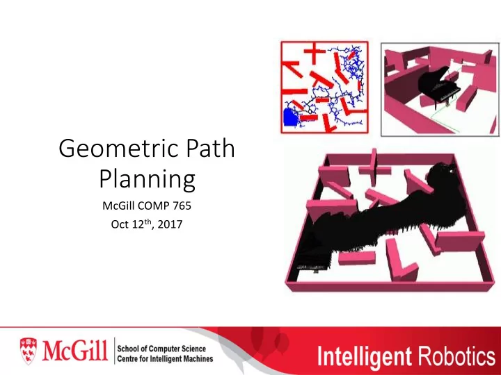
Geometric Path Planning

McGill COMP 765 Oct 12th, 2017

The Motion Planning Problem

• Intuition: Find a safe path/trajectory from start to goal
• More precisely:
• A path is a series of robot configurations (e.g., joint angles, points in x-y-

theta, 6-DOF poses, etc)

• A trajectory is a path indexed by time
• We express safety as a set of constraints (e.g., walls, impassable terrain,

unsafe flight configurations, self-penetration of arm links, etc.)

Planning Algorithm Properties

• We can measure the performance of our planning algorithms in a

number of ways:

• Complete: returns a path if one exists. Variants include:
• Resolution complete
• Probabilistically complete
• Optimal: the path returned is the “best” one under some condition (usually

path length, but we can consider others)

• Computational complexity:
• Measured w.r.t. number of dimensions of configuration space, size of the world, number
• f steps in the returned path, etc.
• Nature of constraints handled:
• Holonomic
• Non-holonomic
• Uncertainty awareness

Challenges for motion planning

• Robots are often high dimensional (e.g., humanoid, robot arm,

quadruped) useful paths can require very many motions, and there can be tight constraints between each location (e.g., piano moving)

• The constraints formed by the robot and its environment do not take

a clean form that we can easily optimize over

• Example: if we have a square obstacle on the 2D plane, what is the shape of

the constraint in the 6 degree-of-freedom joint space of a manipulator?

• Motion planning research:
• One of the oldest topics in robotics
• For many years we did not have efficient algorithms to handle the problems

posed by the hardware – approximations and heuristics were abundant

• Today: recent breakthroughs mean that good libraries exists for many of the

problems of interest. Research on pure geometric planning is slightly less and we are ready to tackle uncertainty, differential control, learned models, etc.

Starting Simple: Breadth-first search planning

• Breadth-first search applied to a discrete planning problem:
• From the start, try every possible action and record the result, along with

book-keeping, in an “open list” (queue)

• Until we reach the goal, pop from the open list, try every possible action, and

place the results back at the end of the open list

• BFS is a complete planner, it explores all possible paths
• It scales very badly with dimension and path length
• Can only handle discrete or discretized environments

A* Planning

• Same structure as BFS, but add a heuristic function that estimates the

cost-to-goal from each location

• The open-list becomes a priority queue on the function:
• 𝑔 𝑜 = 𝑕 𝑜 + ℎ 𝑜
• With g the cost so far and h the heuristic
• The heuristic guides our computation to open nodes in the direction
• f the goal first
• As long as h is admissible (it never over-estimates), we are

guaranteed an optimal solution when we first open the goal

• Still a complete planner as we eventually open all nodes regardless of

h

A-star

• A* is used very often as a long-

term planner in robotics, when the world can be considered discrete and controls are ignored

• Examples:
• Self-driving car routes through city

maps

• Navigation through indoor hallways

Issues with A-star

• Re-using computation:

–In robotics, map is

• ften evolving (D*,

Stentz et al.)

–Same path segments

will be shared by many paths (roadmaps and decompositions, soon) Poor scaling to higher dimensions

Robot-Specific Methods

(4) Roadmap approaches (1) Cell decomposition (2) Potential Fields (3) Bug algorithms

Goal reduce the N-dimensional configuration space to a set of

• ne-D paths to search.

Goal account for all of the free space Goal Create flexible local control strategies Limited knowledge path planning with a behavioral approach

Cell Decomposition Planners

• Basic idea, decompose the overall planning process into local regions
• Simple computations can tell us the path through the region (may or

may not be optimal)

• A global computation can be performed to re-assemble the entire

path, and often we can re-use our local computation for multiple queries

• Examples:
• Voronoi diagrams
• Visibility graphs

The Visibility Graph

• Opened vertices = {start}. Repeat until you’re done:
• Add edges from opened vertices to visible obstacles
• If goal visible from latest vertex added, you’re done.

start goal

Since the map was inC

• space, each line potentially represents part of a path

from the start to the goal.

Potential Field Planners

• A more local and reactive method: utilize the constraints and

information nearby to form a simple local motion decision

• Questions:
• How to formulate these local decisions in a coherent way?
• Can we prove any properties or guarantees about the overall plans?
• Potential fields are an intuitive approach based on the motions of

physical bodies propelled by smooth forces

Potential Field Method

Potential Field (Working Principle)

– The goal location generates an attractive potential – pulling the robot towards the goal – The obstacles generate a repulsive potential – pushing the robot away from the obstacles – The negative gradient of the total potential is treated as a force applied to the robot

• - Let the sum of the forces control the robot

C-obstacles

Local techniques

Potential Field methods

• compute a repulsive force away from obstacles
• compute an attractive force toward the goal

• Compute an attractive force toward the goal

Potential Field Method

C- obstacles Attractive potential

Random search

Random walks

Often combined with potential field methods to escape minima

random walks are not perfect...

“Filling in” local minima

Bug Algorithms

• Idea: can we come up with a

simple set of rules that allow us to perform behavior-based travel to goal (no explicit global plan?)

• Yes: follow the intuition of

human labyrinth solving: “Always turn left”

• For the most part, this works

well, but we can devise adversarial complex obstacles where smarts are needed:

• BUG B approach…

Probabilistic Roadmaps (PRMs)

Kavraki, Latombe, Overmars, Svestka, 1994 Developed for high-dimensional spaces Avoid pitfalls of classical grid search Random sampling of C free Find neighbors of each sample (radius parameter) Local planner attempts connections “Probabilistic completeness" achieved

Other PRM variants: Obstacle-Based PRM (Amato, Wu, 1996); Sensor-based PRM (Yu, Gupta, 1998); Gaussian PRM (Boor, Overmars, van der Stappen, 1999); Medial axis PRMs (Wilmarth, Amato, Stiller, 1999; Pisula, Ho, Lin, Manocha, 2000; Kavraki, Guibas, 2000); Contact space PRM (Ji, Xiao, 2000); Closed-chain PRMs (LaValle, Yakey, Kavraki, 1999; Han, Amato 2000); Lazy PRM (Bohlin, Kavraki, 2000); PRM for changing environments (Leven, Hutchinson, 2000); Visibility PRM (Simeon, Laumond, Nissoux, 2000).

• A point P in C is randomly chosen.
• The nearest vertex in the RRT is selected.
• A new edge is added from this vertex in the

direction of P, at distance

• The further the algorithm goes, the more

space is covered.

Start Goal

Random vertex

We greedily connect the bottom tree to our new vertex

Obstacle found !

Now we swap roles !

Now we swap roles !

We grow the bottom tree

Now we greedily try to connect And we continue…

Connection made !

Now we have a solution !

Last step: path smoothing

Last step: path smoothing

Using RRTs

How can RRTs be used to help find paths?

• Can be used on their own (eventually will get close to the goal)
• Can be used with potential field methods
• Every so often (1 in 20 times), choose the goal to be the

next free-space point chosen

• Bias the random configuration chosen toward the goal.

Additional complexity

Nonholonomic vs. Locally Uncontrollable

Also: moving obstacles dynamic constraints

forward-only left-only car

Conclusion and readings

• RRTs are one of the most attractive planners developed to date
• Much research has been generated from applying them to a variety
• f problems in robotics and AI, beyond simple motion planning
• Next Tuesday, we will read two recent research papers that follow-on

from concepts in optimal control and planning:

• LQR-Trees: Feedback Motion Planning on Sparse Randomized Trees by Russ

Tedrake.

• Sampling-based Algorithms for Optimal Motion Planning by Sertac Karaman

and Emilio Frazzoli.

• Unless presenters appear over the weekend, I will lead the

discussions, but please be prepared with questions!