Gaussian processes for regression, global optimization and set - PowerPoint PPT Presentation

Motivations Reminder The previous example was produced in the framework of an ongoing collaboration with T. Krityakierne (now at Mahidol University, Bangkok), G. Pirot (University of Lausanne), and P . Renard (University of Neuchˆ atel). A few general questions About global optimization: does it converge? Does it parallelize well? Can it be applied in higher dimensions? In noise? ⇒ [Part II] What if the target is not to recover (nearly) optimal points but other quantities such as excursion sets or their measure? david@idiap.ch; ginsbourger@stat.unibe.ch GPs for regression and sequential design 9 / 72

Motivations Reminder The previous example was produced in the framework of an ongoing collaboration with T. Krityakierne (now at Mahidol University, Bangkok), G. Pirot (University of Lausanne), and P . Renard (University of Neuchˆ atel). A few general questions About global optimization: does it converge? Does it parallelize well? Can it be applied in higher dimensions? In noise? ⇒ [Part II] What if the target is not to recover (nearly) optimal points but other quantities such as excursion sets or their measure? ⇒ [Part III] david@idiap.ch; ginsbourger@stat.unibe.ch GPs for regression and sequential design 9 / 72

Motivations Reminder The previous example was produced in the framework of an ongoing collaboration with T. Krityakierne (now at Mahidol University, Bangkok), G. Pirot (University of Lausanne), and P . Renard (University of Neuchˆ atel). A few general questions About global optimization: does it converge? Does it parallelize well? Can it be applied in higher dimensions? In noise? ⇒ [Part II] What if the target is not to recover (nearly) optimal points but other quantities such as excursion sets or their measure? ⇒ [Part III] What kind of mathematical properties of f can be incorporated and or learnt with Gaussian Process approaches? david@idiap.ch; ginsbourger@stat.unibe.ch GPs for regression and sequential design 9 / 72

Motivations Reminder The previous example was produced in the framework of an ongoing collaboration with T. Krityakierne (now at Mahidol University, Bangkok), G. Pirot (University of Lausanne), and P . Renard (University of Neuchˆ atel). A few general questions About global optimization: does it converge? Does it parallelize well? Can it be applied in higher dimensions? In noise? ⇒ [Part II] What if the target is not to recover (nearly) optimal points but other quantities such as excursion sets or their measure? ⇒ [Part III] What kind of mathematical properties of f can be incorporated and or learnt with Gaussian Process approaches? ⇒ [Part IV] david@idiap.ch; ginsbourger@stat.unibe.ch GPs for regression and sequential design 9 / 72

Motivations Reminder The previous example was produced in the framework of an ongoing collaboration with T. Krityakierne (now at Mahidol University, Bangkok), G. Pirot (University of Lausanne), and P . Renard (University of Neuchˆ atel). A few general questions About global optimization: does it converge? Does it parallelize well? Can it be applied in higher dimensions? In noise? ⇒ [Part II] What if the target is not to recover (nearly) optimal points but other quantities such as excursion sets or their measure? ⇒ [Part III] What kind of mathematical properties of f can be incorporated and or learnt with Gaussian Process approaches? ⇒ [Part IV] Let us start by a short reminder about Gaussian Processes. david@idiap.ch; ginsbourger@stat.unibe.ch GPs for regression and sequential design 9 / 72

Motivations Reminder Preliminary: priors on functions? A real-valued random field Z with index set D is a collection of random variables ( Z x ) x ∈ D defined over the same probability space (Ω , A , P ) . david@idiap.ch; ginsbourger@stat.unibe.ch GPs for regression and sequential design 10 / 72

Motivations Reminder Preliminary: priors on functions? A real-valued random field Z with index set D is a collection of random variables ( Z x ) x ∈ D defined over the same probability space (Ω , A , P ) . Such random field are defined through their finite-dimensional distributions, that is joint distributions of random vectors of the form ( Z x 1 , . . . , Z x n ) for any finite set of points { x 1 , . . . , x n } ⊂ D ( n ≥ 1). david@idiap.ch; ginsbourger@stat.unibe.ch GPs for regression and sequential design 10 / 72

Motivations Reminder Preliminary: priors on functions? A real-valued random field Z with index set D is a collection of random variables ( Z x ) x ∈ D defined over the same probability space (Ω , A , P ) . Such random field are defined through their finite-dimensional distributions, that is joint distributions of random vectors of the form ( Z x 1 , . . . , Z x n ) for any finite set of points { x 1 , . . . , x n } ⊂ D ( n ≥ 1). Kolmogorov’s extension theorem tells us that families of joint probability distributions satisfying a few consistency conditions define random fields. david@idiap.ch; ginsbourger@stat.unibe.ch GPs for regression and sequential design 10 / 72

Motivations Reminder Preliminary: priors on functions? A real-valued random field Z with index set D is a collection of random variables ( Z x ) x ∈ D defined over the same probability space (Ω , A , P ) . Such random field are defined through their finite-dimensional distributions, that is joint distributions of random vectors of the form ( Z x 1 , . . . , Z x n ) for any finite set of points { x 1 , . . . , x n } ⊂ D ( n ≥ 1). Kolmogorov’s extension theorem tells us that families of joint probability distributions satisfying a few consistency conditions define random fields. Gaussian Random Fields (GRFs, a.k.a. GPs here) One major example of such family is given by multivariate Gaussian distributions . david@idiap.ch; ginsbourger@stat.unibe.ch GPs for regression and sequential design 10 / 72

Motivations Reminder Preliminary: priors on functions? A real-valued random field Z with index set D is a collection of random variables ( Z x ) x ∈ D defined over the same probability space (Ω , A , P ) . Such random field are defined through their finite-dimensional distributions, that is joint distributions of random vectors of the form ( Z x 1 , . . . , Z x n ) for any finite set of points { x 1 , . . . , x n } ⊂ D ( n ≥ 1). Kolmogorov’s extension theorem tells us that families of joint probability distributions satisfying a few consistency conditions define random fields. Gaussian Random Fields (GRFs, a.k.a. GPs here) One major example of such family is given by multivariate Gaussian distributions . By specifying mean and covariance matrix of random vectors corresponding to any finite set of locations, one defines a GRF / GP . david@idiap.ch; ginsbourger@stat.unibe.ch GPs for regression and sequential design 10 / 72

Motivations Reminder Preliminary: GPs Hence a GP Z is completely defined -as random element over the cylindrical σ algebra of R D - by specifying the mean and the covariance matrix of any random vector of the form ( Z x 1 , . . . , Z x n ) , so that its law is characterized by m : x ∈ D − → m ( x ) = E [ Z x ] ∈ R k : ( x , x ′ ) ∈ D × D − → k ( x , x ′ ) = Cov [ Z x , Z x ′ ] ∈ R david@idiap.ch; ginsbourger@stat.unibe.ch GPs for regression and sequential design 11 / 72

Motivations Reminder Preliminary: GPs Hence a GP Z is completely defined -as random element over the cylindrical σ algebra of R D - by specifying the mean and the covariance matrix of any random vector of the form ( Z x 1 , . . . , Z x n ) , so that its law is characterized by m : x ∈ D − → m ( x ) = E [ Z x ] ∈ R k : ( x , x ′ ) ∈ D × D − → k ( x , x ′ ) = Cov [ Z x , Z x ′ ] ∈ R While m can be any function, k is constrained since ( k ( x i , x j )) 1 ≤ i ≤ n , 1 ≤ j ≤ n must be a covariance matrix, i.e. symmetric positive semi-definite, for any set of points. k satisfying such property are refereed to as p.d. kernels . david@idiap.ch; ginsbourger@stat.unibe.ch GPs for regression and sequential design 11 / 72

Motivations Reminder Preliminary: GPs Hence a GP Z is completely defined -as random element over the cylindrical σ algebra of R D - by specifying the mean and the covariance matrix of any random vector of the form ( Z x 1 , . . . , Z x n ) , so that its law is characterized by m : x ∈ D − → m ( x ) = E [ Z x ] ∈ R k : ( x , x ′ ) ∈ D × D − → k ( x , x ′ ) = Cov [ Z x , Z x ′ ] ∈ R While m can be any function, k is constrained since ( k ( x i , x j )) 1 ≤ i ≤ n , 1 ≤ j ≤ n must be a covariance matrix, i.e. symmetric positive semi-definite, for any set of points. k satisfying such property are refereed to as p.d. kernels . Remark: Assuming µ ≡ 0 for now, k accounts for a number of properties of Z , including pathwise properties , i.e. functional properties of the paths x ∈ D − → Z x ( ω ) ∈ R , for ω ∈ Ω (paths are also called “realizations”, or “trajectories”). david@idiap.ch; ginsbourger@stat.unibe.ch GPs for regression and sequential design 11 / 72

Motivations Reminder Preliminary: Examples of p.d. kernels and GRFs For d = 1 and k ( t , t ′ ) = min ( t , t ′ ) , one gets the Brownian Motion ( W t ) t ∈ [ 0 , 1 ] . Still for d = 1, k ( t , t ′ ) = min ( t , t ′ ) × ( 1 − max ( t , t ′ )) gives the so-called Brownian Bridge, say ( B t ) t ∈ [ 0 , 1 ] . 2 ( | t | 2 H + | t ′ | 2 H − | t − t ′ | 2 H ) is the covariance Also, for H ∈ ( 0 , 1 ) , k ( t , t ′ ) = 1 kernel of the fractional (or “fractal”) Brownian Motion with Hurst coefficient H . david@idiap.ch; ginsbourger@stat.unibe.ch GPs for regression and sequential design 12 / 72

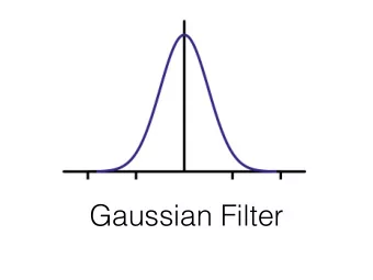
Motivations Reminder Preliminary: Examples of p.d. kernels and GRFs For d = 1 and k ( t , t ′ ) = min ( t , t ′ ) , one gets the Brownian Motion ( W t ) t ∈ [ 0 , 1 ] . Still for d = 1, k ( t , t ′ ) = min ( t , t ′ ) × ( 1 − max ( t , t ′ )) gives the so-called Brownian Bridge, say ( B t ) t ∈ [ 0 , 1 ] . 2 ( | t | 2 H + | t ′ | 2 H − | t − t ′ | 2 H ) is the covariance Also, for H ∈ ( 0 , 1 ) , k ( t , t ′ ) = 1 kernel of the fractional (or “fractal”) Brownian Motion with Hurst coefficient H . k ( t , t ′ ) = e −| t − t ′ | is called exponential kernel and characterizes the Ornstein-Uhlenbeck process . k ( t , t ′ ) = e −| t − t ′ | 2 is the Gaussian kernel. david@idiap.ch; ginsbourger@stat.unibe.ch GPs for regression and sequential design 12 / 72

Motivations Reminder Preliminary: Examples of p.d. kernels and GRFs For d = 1 and k ( t , t ′ ) = min ( t , t ′ ) , one gets the Brownian Motion ( W t ) t ∈ [ 0 , 1 ] . Still for d = 1, k ( t , t ′ ) = min ( t , t ′ ) × ( 1 − max ( t , t ′ )) gives the so-called Brownian Bridge, say ( B t ) t ∈ [ 0 , 1 ] . 2 ( | t | 2 H + | t ′ | 2 H − | t − t ′ | 2 H ) is the covariance Also, for H ∈ ( 0 , 1 ) , k ( t , t ′ ) = 1 kernel of the fractional (or “fractal”) Brownian Motion with Hurst coefficient H . k ( t , t ′ ) = e −| t − t ′ | is called exponential kernel and characterizes the Ornstein-Uhlenbeck process . k ( t , t ′ ) = e −| t − t ′ | 2 is the Gaussian kernel. The two last kernels possess a so-called stationarity (or “shift-invariance”) property. Also, in turns out that these kernels can be generalized to d ≥ 1: k ( x , x ′ ) = e −|| x − x ′ || (“isotropic exponential”) k ( x , x ′ ) = e −|| x − x ′ || 2 (“isotropic Gaussian”) david@idiap.ch; ginsbourger@stat.unibe.ch GPs for regression and sequential design 12 / 72

Motivations Reminder Some GRF R simulations (d=2) with RandomFields david@idiap.ch; ginsbourger@stat.unibe.ch GPs for regression and sequential design 13 / 72

Motivations Reminder Some GRF R simulations (d=1) with DiceKriging Here k ( t , t ′ ) = σ 2 � � 1 + | t ′ − t | /ℓ + ( t − t ′ ) 2 / ( 3 ℓ 2 ) exp ( −| h | /ℓ ) ( Mat´ ern kernel with regularity parameter 5 / 2) where ℓ = 0 . 4 and σ = 1 . 5. Furthermore, here trend is a trend m ( t ) = − 1 + 2 t + 3 t 2 . 6 4 2 z 0 −2 −4 0.0 0.2 0.4 0.6 0.8 1.0 x david@idiap.ch; ginsbourger@stat.unibe.ch GPs for regression and sequential design 14 / 72

Motivations Reminder Properties of GRFs and kernels Back to centred Z for simplicity, one can define a (pseudo-)metric d Z on D by � � d 2 Z ( x , x ′ ) = E ( Z x − Z x ′ ) 2 ) = k ( x , x ) + k ( x ′ , x ′ ) − 2 k ( x , x ′ ) A number of properties of Z are driven by d Z . david@idiap.ch; ginsbourger@stat.unibe.ch GPs for regression and sequential design 15 / 72

Motivations Reminder Properties of GRFs and kernels Back to centred Z for simplicity, one can define a (pseudo-)metric d Z on D by � � d 2 Z ( x , x ′ ) = E ( Z x − Z x ′ ) 2 ) = k ( x , x ) + k ( x ′ , x ′ ) − 2 k ( x , x ′ ) A number of properties of Z are driven by d Z . For instance, Theorem (Sufficient condition for the continuity of GRF paths) Let ( Z x ) x ∈ D be a separable Gaussian random field on a compact index set D ⊂ R d . If for some 0 < C < ∞ and δ, η > 0 , C d 2 Z ( x , x ′ ) ≤ � � � 1 + δ � log || x − x ′ || for all x , x ′ ∈ D with || x − x ′ || < η , then the paths of Z are almost surely continuous and bounded. See, e.g., M. Scheuerer’s PhD thesis (2009) for details. david@idiap.ch; ginsbourger@stat.unibe.ch GPs for regression and sequential design 15 / 72

Motivations Reminder Properties of GRFs and kernels Several other pathwise properties of Z can be controlled through k , such as differentiability, but also symmetries, harmonicity, and more (Cf. Part IV). david@idiap.ch; ginsbourger@stat.unibe.ch GPs for regression and sequential design 16 / 72

Motivations Reminder Properties of GRFs and kernels Several other pathwise properties of Z can be controlled through k , such as differentiability, but also symmetries, harmonicity, and more (Cf. Part IV). In practice, the choice of k often relies (in)directly on Bochner’s theorem. Noting k ( h ) = k ( x , x ′ ) for k stationary and h = x − x ′ , we have david@idiap.ch; ginsbourger@stat.unibe.ch GPs for regression and sequential design 16 / 72

Motivations Reminder Properties of GRFs and kernels Several other pathwise properties of Z can be controlled through k , such as differentiability, but also symmetries, harmonicity, and more (Cf. Part IV). In practice, the choice of k often relies (in)directly on Bochner’s theorem. Noting k ( h ) = k ( x , x ′ ) for k stationary and h = x − x ′ , we have Theorem (Bochner’s theorem) A function k : R d − → R is continuous and positive definite if and only if a finite symmetric non-negative measure ν on R d exists so that � for all h ∈ R d k ( h ) = R d cos ( � h , w � ) ν ( d w ) ν is then called the spectral measure of k. david@idiap.ch; ginsbourger@stat.unibe.ch GPs for regression and sequential design 16 / 72

Motivations Reminder Properties of GRFs and kernels Several other pathwise properties of Z can be controlled through k , such as differentiability, but also symmetries, harmonicity, and more (Cf. Part IV). In practice, the choice of k often relies (in)directly on Bochner’s theorem. Noting k ( h ) = k ( x , x ′ ) for k stationary and h = x − x ′ , we have Theorem (Bochner’s theorem) A function k : R d − → R is continuous and positive definite if and only if a finite symmetric non-negative measure ν on R d exists so that � for all h ∈ R d k ( h ) = R d cos ( � h , w � ) ν ( d w ) ν is then called the spectral measure of k. For ν absolutely continuous with ν = ϕ d Leb d , ϕ is called the spectral density ern ≡ ϕ ( w ) = ( 1 + || w || 2 ) − r . of k . Example: Mat´ david@idiap.ch; ginsbourger@stat.unibe.ch GPs for regression and sequential design 16 / 72

Motivations Reminder Properties of GRFs and kernels Sarting from known d.p. kernels, it is common to enrich the choice by appealing to operations preserving symmetry & positive definiteness, e.g.: Non-negative linear combinations of p.d. kernels Products and tensor products of p.d. kernels Multiplication by σ ( x ) σ ( x ′ ) for σ : x ∈ D − → [ 0 , + ∞ ) Deformations/warpings: k ( g ( x ) , g ( x ′ )) for g : D − → D Convolutions, etc. . . david@idiap.ch; ginsbourger@stat.unibe.ch GPs for regression and sequential design 17 / 72

Motivations Reminder Properties of GRFs and kernels Sarting from known d.p. kernels, it is common to enrich the choice by appealing to operations preserving symmetry & positive definiteness, e.g.: Non-negative linear combinations of p.d. kernels Products and tensor products of p.d. kernels Multiplication by σ ( x ) σ ( x ′ ) for σ : x ∈ D − → [ 0 , + ∞ ) Deformations/warpings: k ( g ( x ) , g ( x ′ )) for g : D − → D Convolutions, etc. . . C. E. Rasmussen and C.K.I. Williams (2006). Gaussian Processes for Machine Learning. Section “making new kernels from old”. MIT Press david@idiap.ch; ginsbourger@stat.unibe.ch GPs for regression and sequential design 17 / 72

Motivations Reminder A few references M.L. Stein (1999). Interpolation of Spatial Data, Some Theory for Kriging. Springer R. Adler and J. Taylor (2007). Random Fields and Geometry. Springer M. Scheuerer (2009). A Comparison of Models and Methods for Spatial Interpolation in Statistics and Numerical Analysis. PhD thesis of Georg-August Universit¨ at G¨ ottingen O. Roustant, D. Ginsbourger, Y. Deville (2012). DiceKriging, DiceOptim: Two R Packages for the Analysis of Computer Experiments by Kriging-Based Metamodeling and Optimization. Journal of Statistical Software, 51(1), 1-55. M. Schlather, A. Malinowski, P . J. Menck, M. Oesting and K. Strokorb (2015). Analysis, Simulation and Prediction of Multivariate Random Fields with Package RandomFields. Journal of Statistical Software, 63, 8, 1-25. david@idiap.ch; ginsbourger@stat.unibe.ch GPs for regression and sequential design 18 / 72

Motivations Reminder A few references B. Rajput and S. Cambanis (1972). Gaussian processes and Gaussian measures. Ann. Math. Statist. 43 (6), 1944-1952. A. O’Hagan (1978). Curve fitting and optimal design for prediction. Journal of the Royal Statistical Society, Series B, 40(1):1-42. H. Omre and K. Halvorsen (1989). The bayesian bridge between simple and universal kriging. Mathematical Geology, 22 (7):767-786. M. S. Handcock and M. L. Stein (1993). A bayesian analysis of kriging. Technometrics, 35(4):403-410. A.W. Van der Vaart and J. H. Van Zanten (2008). Rates of contraction of posterior distributions based on Gaussian process priors. Annals of Statistics, 36:1435-1463. david@idiap.ch; ginsbourger@stat.unibe.ch GPs for regression and sequential design 19 / 72

About the Expected Improvement Some challenging questions Part II About GP-based Bayesian optimization david@idiap.ch; ginsbourger@stat.unibe.ch GPs for regression and sequential design 20 / 72

About the Expected Improvement Some challenging questions Some seminal papers H.J. Kushner (1964). A new method of locating the maximum of an arbitrary multi-peak curve in the presence of noise. Journal of Basic Engineering, 86:97-106. J. Mockus (1972). On Bayesian methods for seeking the extremum. Automatics and Computers (Avtomatika i Vychislitel’naya Tekhnika), 4(1):53-62. J. Mockus, V. Tiesis, and A. Zilinskas (1978). The application of Bayesian methods for seeking the extremum. In Dixon, L. C. W. and Szeg¨ o, G. P ., editors, Towards Global Optimisation, volume 2, pages 117-129. Elsevier Science Ltd., North Holland, Amsterdam. J.M. Calvin (1997). Average performance of a class of adaptive algorithms for global optimization. The Annals of Applied Probability, 7(3):711-730. M. Schonlau, W.J. Welch and D.R. Jones (1998). Efficient Global Optimization of Expensive Black-box Functions. Journal of Global Optimization . david@idiap.ch; ginsbourger@stat.unibe.ch GPs for regression and sequential design 21 / 72

About the Expected Improvement Some challenging questions Decision-theoretic roots of EI (1) Assume that f (modelled by Z ) was already evaluated at a set of points X n = { x 1 , . . . , x n } ⊂ D ( n ≥ n 0 ), at that one wishes to perform additional evaluations at one or more points x n + j ∈ D (1 ≤ j ≤ q , q ≥ 1). david@idiap.ch; ginsbourger@stat.unibe.ch GPs for regression and sequential design 22 / 72

About the Expected Improvement Some challenging questions Decision-theoretic roots of EI (1) Assume that f (modelled by Z ) was already evaluated at a set of points X n = { x 1 , . . . , x n } ⊂ D ( n ≥ n 0 ), at that one wishes to perform additional evaluations at one or more points x n + j ∈ D (1 ≤ j ≤ q , q ≥ 1). A rather natural score to judge performances in minimization at step n is the regret t n − f ⋆ (a.k.a. optimality gap), where t n = min 1 ≤ i ≤ n f ( x i ) . david@idiap.ch; ginsbourger@stat.unibe.ch GPs for regression and sequential design 22 / 72

About the Expected Improvement Some challenging questions Decision-theoretic roots of EI (1) Assume that f (modelled by Z ) was already evaluated at a set of points X n = { x 1 , . . . , x n } ⊂ D ( n ≥ n 0 ), at that one wishes to perform additional evaluations at one or more points x n + j ∈ D (1 ≤ j ≤ q , q ≥ 1). A rather natural score to judge performances in minimization at step n is the regret t n − f ⋆ (a.k.a. optimality gap), where t n = min 1 ≤ i ≤ n f ( x i ) . When choosing x n + j ∈ D (1 ≤ j ≤ q ), we wish them to minimize t n + q − f ⋆ . david@idiap.ch; ginsbourger@stat.unibe.ch GPs for regression and sequential design 22 / 72

About the Expected Improvement Some challenging questions Decision-theoretic roots of EI (1) Assume that f (modelled by Z ) was already evaluated at a set of points X n = { x 1 , . . . , x n } ⊂ D ( n ≥ n 0 ), at that one wishes to perform additional evaluations at one or more points x n + j ∈ D (1 ≤ j ≤ q , q ≥ 1). A rather natural score to judge performances in minimization at step n is the regret t n − f ⋆ (a.k.a. optimality gap), where t n = min 1 ≤ i ≤ n f ( x i ) . When choosing x n + j ∈ D (1 ≤ j ≤ q ), we wish them to minimize t n + q − f ⋆ . Two problems arise: t n + q cannot be known before evaluating f at the new points 1 f ⋆ is generally not known at all 2 david@idiap.ch; ginsbourger@stat.unibe.ch GPs for regression and sequential design 22 / 72

About the Expected Improvement Some challenging questions Decision-theoretic roots of EI (2) Capitalizing quantities where f is replaced by Z , the standard approach to deal with the first problem is to minimize the expected (simple) regret ( x n + 1 , . . . , x n + q ) ∈ D q − → E n [ T n + q − Z ⋆ ] , where E n refers to the expectation conditional on { Z ( X n ) = z n } . david@idiap.ch; ginsbourger@stat.unibe.ch GPs for regression and sequential design 23 / 72

About the Expected Improvement Some challenging questions Decision-theoretic roots of EI (2) Capitalizing quantities where f is replaced by Z , the standard approach to deal with the first problem is to minimize the expected (simple) regret ( x n + 1 , . . . , x n + q ) ∈ D q − → E n [ T n + q − Z ⋆ ] , where E n refers to the expectation conditional on { Z ( X n ) = z n } . That Z ⋆ is unknown can be circumvented since minimizing E n [ T n + q − Z ⋆ ] is equivalent to minimizing E n [ T n + q ] or E n [ T n + q − T n ] . david@idiap.ch; ginsbourger@stat.unibe.ch GPs for regression and sequential design 23 / 72

About the Expected Improvement Some challenging questions Decision-theoretic roots of EI (2) Capitalizing quantities where f is replaced by Z , the standard approach to deal with the first problem is to minimize the expected (simple) regret ( x n + 1 , . . . , x n + q ) ∈ D q − → E n [ T n + q − Z ⋆ ] , where E n refers to the expectation conditional on { Z ( X n ) = z n } . That Z ⋆ is unknown can be circumvented since minimizing E n [ T n + q − Z ⋆ ] is equivalent to minimizing E n [ T n + q ] or E n [ T n + q − T n ] . Besides this, � � + T n − T n + q = T n − min 1 ≤ j ≤ q Z x n + j . david@idiap.ch; ginsbourger@stat.unibe.ch GPs for regression and sequential design 23 / 72

About the Expected Improvement Some challenging questions Decision-theoretic roots of EI (2) Capitalizing quantities where f is replaced by Z , the standard approach to deal with the first problem is to minimize the expected (simple) regret ( x n + 1 , . . . , x n + q ) ∈ D q − → E n [ T n + q − Z ⋆ ] , where E n refers to the expectation conditional on { Z ( X n ) = z n } . That Z ⋆ is unknown can be circumvented since minimizing E n [ T n + q − Z ⋆ ] is equivalent to minimizing E n [ T n + q ] or E n [ T n + q − T n ] . Besides this, � � + T n − T n + q = T n − min 1 ≤ j ≤ q Z x n + j . Hence, minimizing the expected regret is equivalent to maximizing �� � + � T n − min E n 1 ≤ j ≤ q Z x n + j . david@idiap.ch; ginsbourger@stat.unibe.ch GPs for regression and sequential design 23 / 72

About the Expected Improvement Some challenging questions Definition and derivation of EI Setting q = 1, the Expected Improvement criterion at step n is defined as: → EI n ( x ) = E n [( T n − Z x ) + ] . EI n : x ∈ D − david@idiap.ch; ginsbourger@stat.unibe.ch GPs for regression and sequential design 24 / 72

About the Expected Improvement Some challenging questions Definition and derivation of EI Setting q = 1, the Expected Improvement criterion at step n is defined as: → EI n ( x ) = E n [( T n − Z x ) + ] . EI n : x ∈ D − As T n = t n and Z x ∼ N ( m n ( x ) , k n ( x , x )) conditionally on { Z ( X n ) = z n } , � 0 if s n ( x ) = 0 EI n ( x ) = s n ( x ) { u n ( x )Φ( u n ( x )) + φ ( u n ( x )) } else. � k n ( x , x ) and u n ( x ) = ( t n − m n ( x )) / s n ( x ) . where s n ( x ) = david@idiap.ch; ginsbourger@stat.unibe.ch GPs for regression and sequential design 24 / 72

About the Expected Improvement Some challenging questions Definition and derivation of EI Setting q = 1, the Expected Improvement criterion at step n is defined as: → EI n ( x ) = E n [( T n − Z x ) + ] . EI n : x ∈ D − As T n = t n and Z x ∼ N ( m n ( x ) , k n ( x , x )) conditionally on { Z ( X n ) = z n } , � 0 if s n ( x ) = 0 EI n ( x ) = s n ( x ) { u n ( x )Φ( u n ( x )) + φ ( u n ( x )) } else. � k n ( x , x ) and u n ( x ) = ( t n − m n ( x )) / s n ( x ) . where s n ( x ) = N.B.: EI n is a first order moment of a truncated Gaussian. david@idiap.ch; ginsbourger@stat.unibe.ch GPs for regression and sequential design 24 / 72

About the Expected Improvement Some challenging questions Selected properties of the EI criterion EI n is non-negative over D and vanishes at X n 1 2 EI n is generally not convex/concave and highly multi-modal 3 The regularity of EI n is driven by k n more , sampling using EI 4 If k possesses the “No-Empty-Ball” property eventually fills the space provided f belongs to the RKHS of kernel k . david@idiap.ch; ginsbourger@stat.unibe.ch GPs for regression and sequential design 25 / 72

About the Expected Improvement Some challenging questions Selected properties of the EI criterion EI n is non-negative over D and vanishes at X n 1 2 EI n is generally not convex/concave and highly multi-modal 3 The regularity of EI n is driven by k n more , sampling using EI 4 If k possesses the “No-Empty-Ball” property eventually fills the space provided f belongs to the RKHS of kernel k . NB: new convergence results for EI and more are presented in J. Bect, F . Bachoc and D. Ginsbourger (2016). A supermartingale approach to Gaussian process based sequential design of experiments. HAL/Arxiv paper (hal-01351088, Arxiv: 1608.01118). david@idiap.ch; ginsbourger@stat.unibe.ch GPs for regression and sequential design 25 / 72

About the Expected Improvement Some challenging questions Parallelizing EI algorithms with the multipoint EI Extending the standard EI to q > 1 points is of practical interest as it allows distributing EI algorithms over several processors/computers in parallel. david@idiap.ch; ginsbourger@stat.unibe.ch GPs for regression and sequential design 26 / 72

About the Expected Improvement Some challenging questions Parallelizing EI algorithms with the multipoint EI Extending the standard EI to q > 1 points is of practical interest as it allows distributing EI algorithms over several processors/computers in parallel. Efforts have recently been paid to calculate the “multipoint EI” criterion: �� � + � EI n : ( x 1 , . . . , x q ) ∈ D q − → E n T n − min 1 ≤ j ≤ q ( Z x j ) . david@idiap.ch; ginsbourger@stat.unibe.ch GPs for regression and sequential design 26 / 72

About the Expected Improvement Some challenging questions Parallelizing EI algorithms with the multipoint EI Extending the standard EI to q > 1 points is of practical interest as it allows distributing EI algorithms over several processors/computers in parallel. Efforts have recently been paid to calculate the “multipoint EI” criterion: �� � + � EI n : ( x 1 , . . . , x q ) ∈ D q − → E n T n − min 1 ≤ j ≤ q ( Z x j ) . D. Ginsbourger, R. Le Riche, L. Carraro (2010) Kriging is well-suited to parallelize optimization In Computational Intelligence in Expensive Optimization Problems, Adaptation Learning and Optimization, pages 131-162. Springer Berlin Heidelberg, 2010 Goto equations C. Chevalier, D. Ginsbourger (2013) Fast computation of the multipoint Expected Improvement with applications in batch selection. Learning and Intelligent Optimization (LION7) david@idiap.ch; ginsbourger@stat.unibe.ch GPs for regression and sequential design 26 / 72

About the Expected Improvement Some challenging questions Multipoint EI: Example david@idiap.ch; ginsbourger@stat.unibe.ch GPs for regression and sequential design 27 / 72

About the Expected Improvement Some challenging questions Multipoint EI: Latest results and ongoing work The main computational bottleneck lies in the maximization of the Multipoint EI criterion over D q . david@idiap.ch; ginsbourger@stat.unibe.ch GPs for regression and sequential design 28 / 72

About the Expected Improvement Some challenging questions Multipoint EI: Latest results and ongoing work The main computational bottleneck lies in the maximization of the Multipoint EI criterion over D q . Closed formulae as well as fast and efficient approximations have been obtained for the gradient of the multipoint EI criterion. S. Marmin, C. Chevalier, D. Ginsbourger. (2015). Differentiating the multipoint Expected Improvement for optimal batch design. International Workshop on Machine learning, Optimization and big Data. david@idiap.ch; ginsbourger@stat.unibe.ch GPs for regression and sequential design 28 / 72

About the Expected Improvement Some challenging questions Multipoint EI: Latest results and ongoing work The main computational bottleneck lies in the maximization of the Multipoint EI criterion over D q . Closed formulae as well as fast and efficient approximations have been obtained for the gradient of the multipoint EI criterion. S. Marmin, C. Chevalier, D. Ginsbourger. (2015). Differentiating the multipoint Expected Improvement for optimal batch design. International Workshop on Machine learning, Optimization and big Data. S. Marmin, C. Chevalier, D. Ginsbourger. (2016+). Efficient batch-sequential Bayesian optimization with moments of truncated Gaussian vectors. Hal/Arxiv paper (https://hal.archives-ouvertes.fr/hal-01361894/). david@idiap.ch; ginsbourger@stat.unibe.ch GPs for regression and sequential design 28 / 72

About the Expected Improvement Some challenging questions Multipoint EI: Latest results and ongoing work The main computational bottleneck lies in the maximization of the Multipoint EI criterion over D q . Closed formulae as well as fast and efficient approximations have been obtained for the gradient of the multipoint EI criterion. S. Marmin, C. Chevalier, D. Ginsbourger. (2015). Differentiating the multipoint Expected Improvement for optimal batch design. International Workshop on Machine learning, Optimization and big Data. S. Marmin, C. Chevalier, D. Ginsbourger. (2016+). Efficient batch-sequential Bayesian optimization with moments of truncated Gaussian vectors. Hal/Arxiv paper (https://hal.archives-ouvertes.fr/hal-01361894/). N.B.: alternative approaches for maximizing the multipoint EI, that rely on stochastic gradients, have been developed by Peter Frazier and his group. david@idiap.ch; ginsbourger@stat.unibe.ch GPs for regression and sequential design 28 / 72

About the Expected Improvement Some challenging questions On finite-time Bayesian Global Optimization Let us now assume that a fixed number of evaluations (after step n 0 ), say r ≥ 1, is allocated for the sequential minimization of f (one point at a time). By construction, we know that EI is optimal at the last iteration. However, maximizing EI is generally not optimal if there remains more than one step. david@idiap.ch; ginsbourger@stat.unibe.ch GPs for regression and sequential design 29 / 72

About the Expected Improvement Some challenging questions On finite-time Bayesian Global Optimization Let us now assume that a fixed number of evaluations (after step n 0 ), say r ≥ 1, is allocated for the sequential minimization of f (one point at a time). By construction, we know that EI is optimal at the last iteration. However, maximizing EI is generally not optimal if there remains more than one step. There exists in fact an optimal strategy, relying on backward induction. Taking a simple example with r = 2, the optimal action at step n 0 is to maximize �� � + � x − → E n 0 T n 0 − min ( Z x , Z X ∗ 2 ) , where X ∗ 2 maximizes EI n 0 + 1 (and so depends on Z x ). david@idiap.ch; ginsbourger@stat.unibe.ch GPs for regression and sequential design 29 / 72

About the Expected Improvement Some challenging questions On finite-time BO: a few references J. Mockus (1982) The Bayesian approach to global optimization. In Systems Modeling and Optimization, volume 38, pp. 473-481. Springer. M. A. Osborne, R. Garnett, and S.J. Roberts (2009) Gaussian processes for global optimization. Learning and Intelligent OptimizatioN conference (LION3). D. Ginsbourger, R. Le Riche (2010) Towards Gaussian process-based optimization with finite time horizon. mODa 9 Advances in Model-Oriented Design and Analysis, Contributions to Statistics, pages 89-96. Physica-Verlag HD. S. Gr¨ unew¨ alder, J. Y. Audibert, M. Opper, and J. Shawe-Taylor (2010). Goto detail . Regret bounds for Gaussian process bandit problems. In International Conference on Artificial Intelligence and Statistics (pp. 273-280), MIT Press. J. Gonzalez, M. Osborne, N. Lawrence (2016). GLASSES: Relieving The Myopia Of Bayesian Optimisation. In Proceedings of the 19th International Conference on Artificial Intelligence and Statistics (pp. 790-799). david@idiap.ch; ginsbourger@stat.unibe.ch GPs for regression and sequential design 30 / 72

About the Expected Improvement Some challenging questions About (very) high-dimensional BO One of the bottlenecks of Global Optimization is high-dimensionality. How to minimize f when n is severely limited and d is very large? One often (realistically) assume that f only depends on d e << d variables. david@idiap.ch; ginsbourger@stat.unibe.ch GPs for regression and sequential design 31 / 72

About the Expected Improvement Some challenging questions About (very) high-dimensional BO One of the bottlenecks of Global Optimization is high-dimensionality. How to minimize f when n is severely limited and d is very large? One often (realistically) assume that f only depends on d e << d variables. Some attempts have recently been done in Bayesian Optimization, that mostly rely on one of the two following ideas: Trying to identify the subset of d e influential variables Restricting the search to one or more d e -dimensional space(s) via random embedding(s) david@idiap.ch; ginsbourger@stat.unibe.ch GPs for regression and sequential design 31 / 72

About the Expected Improvement Some challenging questions About (very) high-dimensional BO: a few references B. Chen, R.M. Castro, and A. Krause (2012) Joint Optimization and Variable Selection of High-dimensional Gaussian Processes In International Conference on Machine Learning Z. Wang, M. Zoghi, F. Hutter, D. Matheson, and N. de Freitas (2013) Bayesian optimization in a billion dimensions via random embeddings . In International Joint Conferences on Artificial Intelligence J. Djolonga, A. Krause, and V. Cevher (2013). High-Dimensional Gaussian Process Bandits. In Neural Information Processing Systems. M. Binois, D. Ginsbourger, O. Roustant (2015). A warped kernel improving robustness in Bayesian optimization via random embeddings. In Learning and Intelligent Optimization (LION9) M. Binois (2015). Uncertainty quantification on Pareto fronts and high-dimensional strategies in Bayesian optimization, with applications in multi-objective automotive design. Ph.D. thesis, Ecole des Mines de Saint-Etienne. david@idiap.ch; ginsbourger@stat.unibe.ch GPs for regression and sequential design 32 / 72

About the Expected Improvement Some challenging questions Mitigating model uncertainty in BO Model-based criteria such as EI are usually calculated under the assumption that k and/or its parameters is/are known. david@idiap.ch; ginsbourger@stat.unibe.ch GPs for regression and sequential design 33 / 72

About the Expected Improvement Some challenging questions Mitigating model uncertainty in BO Model-based criteria such as EI are usually calculated under the assumption that k and/or its parameters is/are known. Incorporating estimation uncertainty into Bayesian global optimization algorithms has been done using various approaches, including notably Making it ”Full Bayesian” Appealing to parametric bootstrap david@idiap.ch; ginsbourger@stat.unibe.ch GPs for regression and sequential design 33 / 72

About the Expected Improvement Some challenging questions Mitigating model uncertainty in BO Model-based criteria such as EI are usually calculated under the assumption that k and/or its parameters is/are known. Incorporating estimation uncertainty into Bayesian global optimization algorithms has been done using various approaches, including notably Making it ”Full Bayesian” Appealing to parametric bootstrap Calculating EI in this way was reported to favour exploratory behaviours. david@idiap.ch; ginsbourger@stat.unibe.ch GPs for regression and sequential design 33 / 72

About the Expected Improvement Some challenging questions Mitigating model uncertainty in BO: a few references D. Ginsbourger, C. Helbert, L. Carraro (2008). Discrete mixtures of kernels for Kriging-based Optimization. Quality and Reliability Engineering International, 24(6):681-691. R.B. Gramacy , M. Taddy (2010). Categorical inputs, sensitivity analysis, optimization and importance tempering with tgp version 2, an R package for treed Gaussian process models. Journal of Statistical Software, 33(6). J.P .C. Kleijnen, W. van Beers, I. van Nieuwenhuyse (2012). Expected improvement in efficient global optimization through bootstrapped kriging. Journal of Global Optimization, 54(1):59-73. R. Benassi, J. Bect, and E. Vazquez (2012). Bayesian optimization using sequential Monte Carlo. Learning and Intelligent Optimization (LION6). david@idiap.ch; ginsbourger@stat.unibe.ch GPs for regression and sequential design 34 / 72

About the Expected Improvement Some challenging questions Transition A few other topics beyond our scope Multi-objective/constrained/robust Bayesian optimization ⇒ Cf. notably works of Emmerich et al., Picheny et al., Binois et al., F´ eliot et al., etc. david@idiap.ch; ginsbourger@stat.unibe.ch GPs for regression and sequential design 35 / 72

About the Expected Improvement Some challenging questions Transition A few other topics beyond our scope Multi-objective/constrained/robust Bayesian optimization ⇒ Cf. notably works of Emmerich et al., Picheny et al., Binois et al., F´ eliot et al., etc. Multi-fidelity Bayesian optimization ⇒ Cf. notably works of Forrester et al., Le Gratiet et al., Perdikaris et al., etc. david@idiap.ch; ginsbourger@stat.unibe.ch GPs for regression and sequential design 35 / 72

About the Expected Improvement Some challenging questions Transition A few other topics beyond our scope Multi-objective/constrained/robust Bayesian optimization ⇒ Cf. notably works of Emmerich et al., Picheny et al., Binois et al., F´ eliot et al., etc. Multi-fidelity Bayesian optimization ⇒ Cf. notably works of Forrester et al., Le Gratiet et al., Perdikaris et al., etc. here . A few references about the noisy aspect can be found david@idiap.ch; ginsbourger@stat.unibe.ch GPs for regression and sequential design 35 / 72

About the Expected Improvement Some challenging questions Transition A few other topics beyond our scope Multi-objective/constrained/robust Bayesian optimization ⇒ Cf. notably works of Emmerich et al., Picheny et al., Binois et al., F´ eliot et al., etc. Multi-fidelity Bayesian optimization ⇒ Cf. notably works of Forrester et al., Le Gratiet et al., Perdikaris et al., etc. here . A few references about the noisy aspect can be found Note also that beyond EI, further criteria are in use for Bayesian optimization and related. Upper Confidence Bound strategies are quite popular, notably as they lead to elegant theoretical results; See e.g. works by Andreas Krause and team, and also recent contributions by Emile Contal et al. david@idiap.ch; ginsbourger@stat.unibe.ch GPs for regression and sequential design 35 / 72

Stepwise Uncertainty Reduction Towards conservative excursion set estimation Part III On the estimation of excursion sets and their measure, and stepwise uncertainty reduction david@idiap.ch; ginsbourger@stat.unibe.ch GPs for regression and sequential design 36 / 72

Stepwise Uncertainty Reduction Towards conservative excursion set estimation Background and motivations A number of practical problems boil down to determining sets of the form Γ ⋆ = { x ∈ D : f ( x ) ∈ T } = f − 1 ( T ) where D is a compact subset of R d ( d ≥ 1), f : D − → R k ( k ≥ 1) is a ( B ( D ) , B ( R k )) -measurable function, and T ∈ B ( R k ) . david@idiap.ch; ginsbourger@stat.unibe.ch GPs for regression and sequential design 37 / 72

Stepwise Uncertainty Reduction Towards conservative excursion set estimation Background and motivations A number of practical problems boil down to determining sets of the form Γ ⋆ = { x ∈ D : f ( x ) ∈ T } = f − 1 ( T ) where D is a compact subset of R d ( d ≥ 1), f : D − → R k ( k ≥ 1) is a ( B ( D ) , B ( R k )) -measurable function, and T ∈ B ( R k ) . For simplicity, we essentially focus today on the case where k = 1, f is continuous, and T = [ t , + ∞ ) for some prescribed t ∈ R . Γ ⋆ = { x ∈ D : f ( x ) ≥ t } is then referred to as the excursion set of f above t . david@idiap.ch; ginsbourger@stat.unibe.ch GPs for regression and sequential design 37 / 72

Stepwise Uncertainty Reduction Towards conservative excursion set estimation Background and motivations A number of practical problems boil down to determining sets of the form Γ ⋆ = { x ∈ D : f ( x ) ∈ T } = f − 1 ( T ) where D is a compact subset of R d ( d ≥ 1), f : D − → R k ( k ≥ 1) is a ( B ( D ) , B ( R k )) -measurable function, and T ∈ B ( R k ) . For simplicity, we essentially focus today on the case where k = 1, f is continuous, and T = [ t , + ∞ ) for some prescribed t ∈ R . Γ ⋆ = { x ∈ D : f ( x ) ≥ t } is then referred to as the excursion set of f above t . Our aim is to estimate Γ ⋆ and quantify uncertainty on it when f can solely be evaluated at a few points X n = { x 1 , . . . , x n } ⊂ D . david@idiap.ch; ginsbourger@stat.unibe.ch GPs for regression and sequential design 37 / 72

Stepwise Uncertainty Reduction Towards conservative excursion set estimation Test case from safety engineering Figure: Excursion set (light gray) of a nuclear criticality safety coefficient depending on two design parameters. Blue triangles: initial experiments. C. Chevalier (2013). Fast uncertainty reduction strategies relying on Gaussian process models. Ph.D. thesis, University of Bern. david@idiap.ch; ginsbourger@stat.unibe.ch GPs for regression and sequential design 38 / 72

Stepwise Uncertainty Reduction Towards conservative excursion set estimation Making a sensible estimation of Γ ⋆ based on a drastically limited number of evaluations f ( X n ) = ( f ( x 1 ) , . . . , f ( x n )) ′ calls for additional assumptions on f . david@idiap.ch; ginsbourger@stat.unibe.ch GPs for regression and sequential design 39 / 72

Stepwise Uncertainty Reduction Towards conservative excursion set estimation Making a sensible estimation of Γ ⋆ based on a drastically limited number of evaluations f ( X n ) = ( f ( x 1 ) , . . . , f ( x n )) ′ calls for additional assumptions on f . In the GP set-up, the main object of interest is represented by Γ = { x ∈ D : Z ( x ) ∈ T } = Z − 1 ( T ) Under our previous assumptions on T (and assuming that is chosen Z with continuous paths a.s.), Γ appears to be a Random Closed Set. david@idiap.ch; ginsbourger@stat.unibe.ch GPs for regression and sequential design 39 / 72

Stepwise Uncertainty Reduction Towards conservative excursion set estimation Simulating excursion sets under a GRF model Several realizations of Γ simulated on a grid 50 × 50 knowing Z ( X n ) = f ( X n ) . david@idiap.ch; ginsbourger@stat.unibe.ch GPs for regression and sequential design 40 / 72

Stepwise Uncertainty Reduction Towards conservative excursion set estimation Kriging (Gaussian Process Interpolation) � m n ( x ) = m ( x ) + k ( X n , x ) T k ( X n , X n ) − 1 ( f ( X n ) − m ( X n )) s 2 n ( x ) = k ( x , x ) − k ( X n , x ) T k ( X n , X n ) − 1 k ( X n , x ) david@idiap.ch; ginsbourger@stat.unibe.ch GPs for regression and sequential design 41 / 72

Stepwise Uncertainty Reduction Towards conservative excursion set estimation � � m n ( x ) − t p n ( x ) = P n ( x ∈ Γ ) = P n ( Z ( x ) ≥ t ) = Φ s n ( x ) david@idiap.ch; ginsbourger@stat.unibe.ch GPs for regression and sequential design 42 / 72

Stepwise Uncertainty Reduction Towards conservative excursion set estimation SUR strategies for inversion and related problems Let us focus first on estimating the measure of excursion α ⋆ := µ ( Γ ⋆ ) where µ is some prescribed finite measure on ( D , B ( D )) . david@idiap.ch; ginsbourger@stat.unibe.ch GPs for regression and sequential design 43 / 72

Stepwise Uncertainty Reduction Towards conservative excursion set estimation SUR strategies for inversion and related problems Let us focus first on estimating the measure of excursion α ⋆ := µ ( Γ ⋆ ) where µ is some prescribed finite measure on ( D , B ( D )) . Defining α := µ ( Γ ) , a number of quantities involving the distribution of α conditional on Z ( x 1 ) , . . . Z ( x n ) can be calculated (in particular moments). david@idiap.ch; ginsbourger@stat.unibe.ch GPs for regression and sequential design 43 / 72

Stepwise Uncertainty Reduction Towards conservative excursion set estimation SUR strategies for inversion and related problems Let us focus first on estimating the measure of excursion α ⋆ := µ ( Γ ⋆ ) where µ is some prescribed finite measure on ( D , B ( D )) . Defining α := µ ( Γ ) , a number of quantities involving the distribution of α conditional on Z ( x 1 ) , . . . Z ( x n ) can be calculated (in particular moments). Approach considered here: sequentially reducing the excursion volume variance thanks to Stepwise Uncertainty Reduction (SUR) strategies david@idiap.ch; ginsbourger@stat.unibe.ch GPs for regression and sequential design 43 / 72

Stepwise Uncertainty Reduction Towards conservative excursion set estimation SUR strategies for inversion and related problems We consider 1-step-lookahead optimal SUR strategies: Define a notion of uncertainty at time n : H n ≥ 0 (e.g., var n ( α ) ). Reduce this uncertainty by evaluating Z at new points Sequential settings: evaluate sequentially the location x ⋆ n + 1 minimizing the so-called SUR criterion associated with H n : J n ( x n + 1 ) := E n ( H n + 1 ( x n + 1 )) david@idiap.ch; ginsbourger@stat.unibe.ch GPs for regression and sequential design 44 / 72

Stepwise Uncertainty Reduction Towards conservative excursion set estimation SUR strategies for inversion and related problems We consider 1-step-lookahead optimal SUR strategies: Define a notion of uncertainty at time n : H n ≥ 0 (e.g., var n ( α ) ). Reduce this uncertainty by evaluating Z at new points Sequential settings: evaluate sequentially the location x ⋆ n + 1 minimizing the so-called SUR criterion associated with H n : J n ( x n + 1 ) := E n ( H n + 1 ( x n + 1 )) See notably the following paper and seminal references therein: J. Bect, D. Ginsbourger, L. Li, V. Picheny and E. Vazquez. Sequential design of computer experiments for the estimation of a probability of failure. Statistics and Computing, 22(3):773-793, 2012. david@idiap.ch; ginsbourger@stat.unibe.ch GPs for regression and sequential design 44 / 72

Stepwise Uncertainty Reduction Towards conservative excursion set estimation SUR strategies: Two candidate uncertainties Two possible definitions for the uncertainty H n are considered here: H n := V ar n ( α ) � � H n := p n ( 1 − p n ) d µ D david@idiap.ch; ginsbourger@stat.unibe.ch GPs for regression and sequential design 45 / 72

Stepwise Uncertainty Reduction Towards conservative excursion set estimation SUR strategies: Two candidate uncertainties Two possible definitions for the uncertainty H n are considered here: H n := V ar n ( α ) � � H n := p n ( 1 − p n ) d µ D Uncertainties: SUR criteria: J n ( x ) := E n ( V ar n + 1 ( α )) H n := V ar n ( α ) � �� � � � H n := p n ( 1 − p n ) d µ p n + 1 ( 1 − p n + 1 ) d µ J n ( x ) := E n X D Main challenge to calculate � J n ( x ) (similar for J n ( x ) ): Obtain a closed form expression for E n ( p n + 1 ( 1 − p n + 1 )) and integrate it. david@idiap.ch; ginsbourger@stat.unibe.ch GPs for regression and sequential design 45 / 72

Stepwise Uncertainty Reduction Towards conservative excursion set estimation Deriving SUR criteria Proposition � � � � � � a ( x ) c ( x ) 1 − c ( x ) E n ( p n + 1 ( x )( 1 − p n + 1 ( x ))) = Φ 2 , − a ( x ) 1 − c ( x ) c ( x ) • Φ 2 ( · , M ) : c.d.f. of centred bivariate Gaussian with covariance matrix M • a ( x ) := ( m n ( x ) − t ) / s n + q ( x ) , c ( x ) := s 2 n ( x ) / s 2 • n + q ( x ) C. Chevalier, J. Bect, D. Ginsbourger, V. Picheny, E. Vazquez and Y. Richet. Fast parallel kriging-based stepwise uncertainty reduction with application to the identification of an excursion set. Technometrics, 56(4):455-465, 2014. david@idiap.ch; ginsbourger@stat.unibe.ch GPs for regression and sequential design 46 / 72