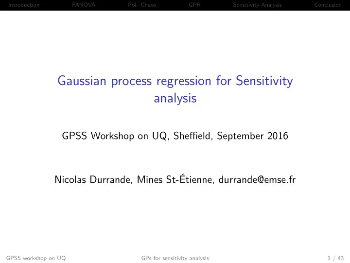
Gaussian process regression for Sensitivity analysis GPSS Workshop - PowerPoint PPT Presentation

Introduction FANOVA Pol. Chaos GPR Sensitivity Analysis Conclusion Gaussian process regression for Sensitivity analysis GPSS Workshop on UQ, Sheffield, September 2016 Nicolas Durrande, Mines St-Étienne, durrande@emse.fr GPSS workshop on UQ GPs for sensitivity analysis 1 / 43

Introduction FANOVA Pol. Chaos GPR Sensitivity Analysis Conclusion Introduction FANOVA, ie HDMR, ie Sobol-Hoeffding representation Polynomial Chaos Gaussian process Regression Sensitivity Analysis Conclusion GPSS workshop on UQ GPs for sensitivity analysis 2 / 43

Introduction FANOVA Pol. Chaos GPR Sensitivity Analysis Conclusion We assume we are interested in a function f : R d → R with d ≥ 2. We want to get some understanding on the “structure” of f : What is the effect of each input variables on the output ? Do some variables have more influence than other ? Do some variables interact together ? The talk will be illustrated on the following test function : f : [0 , 1] 6 → R x �→ 10 sin( π x 1 x 2 ) + 20( x 3 − 0 . 5) 2 + 10 x 4 + 5 x 5 GPSS workshop on UQ GPs for sensitivity analysis 3 / 43

Introduction FANOVA Pol. Chaos GPR Sensitivity Analysis Conclusion First thing one can do is to plot the output versus each input. For 100 samples uniformly distributed over [0 , 1] 6 we get : 25 20 15 10 5 x 1 x 2 x 3 0 25 20 15 10 5 x 4 x 5 x 6 0 0.0 0.2 0.4 0.6 0.8 1.0 0.0 0.2 0.4 0.6 0.8 1.0 0.0 0.2 0.4 0.6 0.8 1.0 GPSS workshop on UQ GPs for sensitivity analysis 4 / 43

Introduction FANOVA Pol. Chaos GPR Sensitivity Analysis Conclusion In a similar fashion, we can fix all variables except one. In graph bellow, all non plotted variables are set to 0 . 5. 25 20 15 10 5 x 1 x 2 x 3 0 25 20 15 10 5 x 4 x 5 x 6 0 0.0 0.2 0.4 0.6 0.8 1.0 0.0 0.2 0.4 0.6 0.8 1.0 0.0 0.2 0.4 0.6 0.8 1.0 GPSS workshop on UQ GPs for sensitivity analysis 5 / 43

Introduction FANOVA Pol. Chaos GPR Sensitivity Analysis Conclusion In order to get an insight on the interaction between variables, we can look at the influence of changing the reference value. 30 x 2 = 0 x 2 = 0 . 5 x 2 = 0 x 2 = 0 . 5 x 2 = 0 . 2 x 2 = 0 . 7 x 2 = 0 . 2 x 2 = 0 . 7 25 x 2 = 0 . 4 x 2 = 0 . 9 x 2 = 0 . 4 x 2 = 0 . 9 20 15 10 5 x 1 x 4 0 0.0 0.2 0.4 0.6 0.8 1.0 0.0 0.2 0.4 0.6 0.8 1.0 GPSS workshop on UQ GPs for sensitivity analysis 6 / 43

Introduction FANOVA Pol. Chaos GPR Sensitivity Analysis Conclusion Introduction FANOVA, ie HDMR, ie Sobol-Hoeffding representation Polynomial Chaos Gaussian process Regression Sensitivity Analysis Conclusion GPSS workshop on UQ GPs for sensitivity analysis 7 / 43

Introduction FANOVA Pol. Chaos GPR Sensitivity Analysis Conclusion One common tool for analysing the structure of f is to look at its FANOVA representation : d � � f ( x ) = f 0 + f i ( x i ) + f i , j ( x i , x j ) + · · · + f 1 ,..., d ( x ) i =1 i < j This decomposition is such that : f 0 accounts for the constant term ⇒ all f I are zero mean ( I � = 0) f 1 accounts for all signal that can be explained just by x 1 � ⇒ f I ( x ) dx − 1 = 0 for all I / ∈ { 0 , 1 } � ⇒ f I ( x ) dx 1 = 0 for all I ⊃ 1 In other words, this decomposition is such that all terms are orthogonal in L 2 . GPSS workshop on UQ GPs for sensitivity analysis 8 / 43

Introduction FANOVA Pol. Chaos GPR Sensitivity Analysis Conclusion The expressions of the f I are : � f 0 = f ( x ) d x � f i ( x i ) = f ( x ) d x − i − f 0 � f i , j ( x i , x j ) = f ( x ) d x − ij − f i ( x i ) − f j ( x j ) + f 0 It can also be interesting to look at the total effect of some inputs : � ˜ f 1 ( x 1 ) = f ( x ) d x − 1 � ˜ f 1 , 2 ( x 1 , x 2 ) = f ( x ) d x −{ 1 , 2 } GPSS workshop on UQ GPs for sensitivity analysis 9 / 43

Introduction FANOVA Pol. Chaos GPR Sensitivity Analysis Conclusion On the previous example we obtain : 4 2 0 -2 x 1 x 2 x 3 -4 4 2 0 -2 -4 x 4 x 5 x 6 0.0 0.2 0.4 0.6 0.8 1.0 0.0 0.2 0.4 0.6 0.8 1.0 0.0 0.2 0.4 0.6 0.8 1.0 GPSS workshop on UQ GPs for sensitivity analysis 10 / 43

Introduction FANOVA Pol. Chaos GPR Sensitivity Analysis Conclusion We can also look at 2nd order interactions f 1 , 2 ( x 1 , x 2 ) f 1 , 3 ( x 1 , x 3 ) Interaction x 1 , x 2 Interaction x 1 , x 3 GPSS workshop on UQ GPs for sensitivity analysis 11 / 43

Introduction FANOVA Pol. Chaos GPR Sensitivity Analysis Conclusion The total effect of ( x 1 , x 2 ) is thus ˜ f 1 , 2 ( x 1 , x 2 ) = f 0 + f 1 ( x 1 ) + f 2 ( x 2 ) + f 1 , 2 ( x 1 , x 2 ) GPSS workshop on UQ GPs for sensitivity analysis 12 / 43

Introduction FANOVA Pol. Chaos GPR Sensitivity Analysis Conclusion In practical application f is not analytical so the above method require numerical computations of the integrals. If there is a cost associated with the evaluation of f , surrogate models are useful. Some models are naturally easy to interpret, for example m ( x ) = β 0 + β 1 x 1 + β 2 x 2 but it soon becomes more tricky. m ( x ) = β 0 + β 1 x 1 + β 2 x 2 + β 1 , 2 x 1 x 2 GPSS workshop on UQ GPs for sensitivity analysis 13 / 43

Introduction FANOVA Pol. Chaos GPR Sensitivity Analysis Conclusion In GPR, the mean can be seen either as a linear combination of the observations : m ( x ) = α t F the kernel evaluated at X : m ( x ) = k ( x , X ) β For example, we have for a squared exponential kernel 3.0 3 2.5 Z ( x ) | Z ( X ) = F 2 2.0 k ( x, X ) 1 1.5 0 1.0 -1 0.5 -2 0.0 -0.5 0.0 0.5 1.0 1.5 -0.5 0.0 0.5 1.0 1.5 x x The basis function have a local influence which makes the interpretation difficult. GPSS workshop on UQ GPs for sensitivity analysis 14 / 43

Introduction FANOVA Pol. Chaos GPR Sensitivity Analysis Conclusion Introduction FANOVA, ie HDMR, ie Sobol-Hoeffding representation Polynomial Chaos Gaussian process Regression Sensitivity Analysis Conclusion GPSS workshop on UQ GPs for sensitivity analysis 15 / 43

Introduction FANOVA Pol. Chaos GPR Sensitivity Analysis Conclusion The principle of polynomial chaos is to project f onto a basis of orthonormal polynomials. One dimension For x ∈ R , the h i are of order i . Starting from the constant function h 0 = 1, the following ones can be obtain using Gram-Schmidt orthogonalisation. x 2 − � x , h 0 � h 0 − � x , h 1 � h 1 1 x − � x , h 0 � h 0 h 0 ( x ) = || 1 || , h 1 ( x ) = || x − � x , h 0 � h 0 || , h 2 ( x ) = || x 2 − � x , h 0 � h 0 − � x , h 1 � h 1 || d -dimension In R d , the basis is obtained by a tensor product of one dimensional basis. For example, if d = 2 : h 11 ( x ) = h 1 ( x 1 ) × h 1 ( x 2 ) h 00 ( x ) = 1 × 1 h 20 ( x ) = h 2 ( x 1 ) × 1 h 10 ( x ) = h 1 ( x 1 ) × 1 . . . . h 01 ( x ) = 1 × h 1 ( x 2 ) . = . GPSS workshop on UQ GPs for sensitivity analysis 16 / 43

Introduction FANOVA Pol. Chaos GPR Sensitivity Analysis Conclusion The orthonormal basis H depends on the measure over the input space D . A uniform measure over D = [ − 1 , 1] gives the Legendre basis : h 3 ( x ) = 7 / 4 (5 x 3 − 3 x ) h 0 ( x ) = 1 / 2 h 4 ( x ) = 9 / 16 (35 x 4 − 30 x 2 + 3) h 1 ( x ) = 3 / 2 x . . h 2 ( x ) = 5 / 4 (3 x 2 − 1) . . . = . A standard Gaussian measure over R gives the Hermite basis : √ √ 2 π ) ( x 3 − 3 x ) h 3 ( x ) = 1 / (6 h 0 ( x ) = 1 / 2 π √ √ 2 π ) ( x 4 − 6 x 2 + 3) h 4 ( x ) = 1 / (24 h 1 ( x ) = 1 / 2 π x √ . . 2 π ) ( x 2 − 1) . . h 2 ( x ) = 1 / (2 . = . GPSS workshop on UQ GPs for sensitivity analysis 17 / 43

Introduction FANOVA Pol. Chaos GPR Sensitivity Analysis Conclusion Legendre basis in 1D x 4 4 x 3 x 2 2 x 1 x 0 0 -2 -1.0 -0.5 0.0 0.5 1.0 GPSS workshop on UQ GPs for sensitivity analysis 18 / 43

Introduction FANOVA Pol. Chaos GPR Sensitivity Analysis Conclusion Legendre basis in 2D h 00 h 10 h 01 x 2 x 2 x 2 x 1 x 1 x 1 h 11 h 20 h 21 x 2 x 2 x 2 x 1 x 1 x 1 GPSS workshop on UQ GPs for sensitivity analysis 19 / 43

Introduction FANOVA Pol. Chaos GPR Sensitivity Analysis Conclusion If we consider linear regression model based on polynomial chaos basis functions � m ( x ) = β h I ( x ) I ⊂{ 0 ,... p } the FANOVA representation of m is straightforward. For example in 2D : �� � m 0 = m ( x ) dx 1 dx 2 = β 00 h 00 ( x ) dx 1 dx 2 = β 00 � m 1 ( x 1 ) = m ( x ) dx 2 − m 0 � = β 00 h 00 ( x ) + β 10 h 10 ( x ) + β 20 h 20 ( x ) dx 2 − m 0 = β 10 h 10 ( x 1 ) + β 20 h 20 ( x 1 ) m 1 , 2 ( x ) = ... = β 11 h 11 ( x ) + β 12 h 12 ( x ) + β 21 h 21 ( x ) + β 22 h 22 ( x ) GPSS workshop on UQ GPs for sensitivity analysis 20 / 43

Introduction FANOVA Pol. Chaos GPR Sensitivity Analysis Conclusion We obtain on the motivating example : 6 4 2 0 -2 -4 x 1 x 2 x 3 -6 6 4 2 0 -2 -4 x 4 x 5 x 6 -6 0.0 0.2 0.4 0.6 0.8 1.0 0.0 0.2 0.4 0.6 0.8 1.0 0.0 0.2 0.4 0.6 0.8 1.0 GPSS workshop on UQ GPs for sensitivity analysis 21 / 43

Introduction FANOVA Pol. Chaos GPR Sensitivity Analysis Conclusion Same figure without cheating : 6 4 2 0 -2 -4 x 1 x 2 x 3 -6 6 4 2 0 -2 -4 x 4 x 5 x 6 -6 0.0 0.2 0.4 0.6 0.8 1.0 0.0 0.2 0.4 0.6 0.8 1.0 0.0 0.2 0.4 0.6 0.8 1.0 GPSS workshop on UQ GPs for sensitivity analysis 22 / 43