Gas plume species identification by regression analyses Dave - PowerPoint PPT Presentation
Gas plume species identification by regression analyses Dave Pogorzala May 12, 2004 . I . T R . I . R . I . T T R Digital Imaging and Remote Sensing Laboratory 2 Introduction the RIT Gas Problem Detection does this pixel
Gas plume species identification by regression analyses Dave Pogorzala May 12, 2004 . I . T R . I . R . I . T T R Digital Imaging and Remote Sensing Laboratory
2 Introduction – the RIT Gas Problem • Detection – does this pixel contain a plume? • Identification this research – if so, which gases are in the plume? • Quantification – what is the mixing ratio or column density of these gases? . I . T R . I . R . I . T T R Digital Imaging and Remote Sensing Laboratory
3 Overview • Data • Stepwise regression • Radiance model • Results • Conclusions . I . T R . I . R . I . T T R Digital Imaging and Remote Sensing Laboratory
4 Data Sources Test Image – DIRSIG image – two plumes – one gas per plume – Freon-114 and NH 3 – plumes do not overlap – complex background – 128 bands – 7.5 - 13.6 µm – SEBASS band centers – 10.73 µm . I . T R . I . R . I . T T R Digital Imaging and Remote Sensing Laboratory
5 Data Sources Test Image – DIRSIG image – two plumes – one gas per plume – Freon-114 and NH 3 – plumes do not overlap – complex background – 128 bands NH 3 – 7.5 - 13.6 µm Freon-114 – SEBASS band centers – 10.73 µm . I . T R . I . R . I . T T R Digital Imaging and Remote Sensing Laboratory
6 Data Sources PNNL Gas Spectra – used to create DIRSIG image – used to populate basis vector library – our subset contains 30 gases – most measured at 3 temps: 5, 25 and 50 o C – basis vector library contains 88 gas spectra . I . T R . I . R . I . T T R Digital Imaging and Remote Sensing Laboratory
7 Overview • Data • Stepwise regression • Radiance model • Results • Conclusions . I . T R . I . R . I . T T R Digital Imaging and Remote Sensing Laboratory
8 Stepwise Regression • Stepwise regression is an iterative approach that selects only those basis vectors that contribute to the fit. • This eliminates needless vectors from the model that have insignificant abundances. • In applying this to the gas problem, we begin with a set of vectors that include all possible gases. The hope is that only those gases contained in the plume will be found by the regression. • This allows us to identify gases without prior knowledge of which are present. . I . T R . I . R . I . T T R Digital Imaging and Remote Sensing Laboratory
9 Stepwise Regression Formulate regression as: = + x Af ε ( ) = × x J 1 pixel vector ( ) = × A J N matrix of basis vectors ( ) = × f N 1 vector of abundances = ε error vect or = J 128 bands = N number of basis vectors currently in model = M total available basis vectors . I . T R . I . R . I . T T R Digital Imaging and Remote Sensing Laboratory
10 Stepwise Regression • Determining whether or not to keep a vector in A is done by an F -test (calculated at a probability of 0.99) based on the Analysis of Variance (ANOVA). • ANOVA compares the Sum of Squares due to Regression (SSR) from the N element model to the N -1 element model (primed quantities denote a transpose). ′ ′ = f A x SSR N ′ ′ = SSR f A x − − − N 1 N 1 N 1 . I . T R . I . R . I . T T R Digital Imaging and Remote Sensing Laboratory
11 Stepwise Regression • If the difference between these two SSRs is more significant than the Sum of Squares about Regression (SSE) normalized by its degrees of freedom (its Mean Squared Error, MSE), then the vector is added. ′ ′ ′ = − = − x x f A x SSE total SS SSR SSE = MSE dof • The difference is significant if it’s ratio over the MSE is greater than the F-statistic ′ ′ ′ ′ − f A x f A x > − − − N 1 N 1 F stat MSE . I . T R . I . R . I . T T R Digital Imaging and Remote Sensing Laboratory
12 Overview • Data • Stepwise regression • Radiance model • Results • Conclusions . I . T R . I . R . I . T T R Digital Imaging and Remote Sensing Laboratory
13 Radiance Model • Neglecting atmospheric effects, we can express a plume pixel as: − ( ) ( ) ∑ D D ( ) C ( ) ( ) ( ) ∑ ∑ λ = β ε λ λ λ + λ λ L B , T 1 c k c k B , T j j s i i i i p = j 1 = = i 0 i 0 ( ) λ = L pixel spectrum C ( ) ( ) β ε λ λ = ∑ B , T self - emitted surface radiance j j s = j 1 = c column density of gas i i ( ) λ = k absorption spectrum of gas i i ( ) ( ) D ∑ λ λ = c k B , T self - emitted plume radiance i i p = i 0 . I . T R . I . R . I . T T R Digital Imaging and Remote Sensing Laboratory
14 Radiance Model • We would like to account for plume emission/absorption. – The plume is in emission when T p > T s , absorption when T p < T s . 1. Begin by inverting the background radiance term to solve for a spectral brightness temperature. This is done on a per-pixel basis. ˆ T 2. The maximum of this is the surface temperature estimate, ( ) s , x , y 3. Define five values of ∆ T : -10, -5, 0, 5 and 10 ˆ = ± ∆ T T T 4. Rewrite T p as: ( ) p s , x , y . I . T R . I . R . I . T T R Digital Imaging and Remote Sensing Laboratory
15 Radiance Model • Substituting the temperature contrast term in for T p , we arrive at the final radiance model: [ ] ( ) D ( ) ) ( ) ( ) ) ( ) ∑ ˆ λ − λ = λ λ ± ∆ − λ L L c k B , T T L ( ( ) ( x , y i i s , x , y x , y = i 0 • This can be related to the regression model defined earlier: ( ) ) ( ) → λ − λ x L L ( x , y [ ] ( ) ( ) ) ( ) ˆ → λ λ ± ∆ − λ A k B , T T L ( ) ( i s , x , y x , y → f c i • M is now (88 PNNL spectra)(5 ∆ T va l ues) = 440 basis vectors . I . T R . I . R . I . T T R Digital Imaging and Remote Sensing Laboratory
16 Overview • Data • Stepwise regression • Radiance model • Results • Conclusions . I . T R . I . R . I . T T R Digital Imaging and Remote Sensing Laboratory
17 Results • Stepwise regression was performed on each plume pixel • A binary image cube 256 x 256 x 440 was created – one “map” per basis vector • The basis vectors found by the regression are denoted by turning “on” the pixel (x,y) in each corresponding map. • The 440 maps were then collapsed down to 30, one map per gas species. . I . T R . I . R . I . T T R Digital Imaging and Remote Sensing Laboratory
18 Results • Detection maps for Freon-114 along with the “top 11” false alarms 1. Freon-114 2. Phosgene (phg) 3. Trichloroethylene (tce) 4. Dibromoethane (edb) 5. Sulfur Dioxide (SO 2 ) 6. Hydrazine (hyd) 7. Vinyl Chloride (vcl) 8. Benzene (C 6 H 6 ) 9. Formaldehyde (HCHO) 10. Dichloropropane (dclp-13) 11. Carbon Monoxide (CO) 12. Methane (CH 4 ) . I . T R . I . R . I . T T R Digital Imaging and Remote Sensing Laboratory
19 Results • Detection maps for Ammonia along with the “top 3” false alarms 1. Ammonia (NH 3 ) 2. Hydrazine (hyd) 3. Freon-12 (f12) 4. Acrolein (acrol) . I . T R . I . R . I . T T R Digital Imaging and Remote Sensing Laboratory
20 Results . I . T R . I . R . I . T T R Digital Imaging and Remote Sensing Laboratory
21 Results . I . T R . I . R . I . T T R Digital Imaging and Remote Sensing Laboratory
22 Results • False detections are attributed to spectral overlap of key absorption features. • Magnitude of absorption features are not important since the stepwise regression was unconstrained. – Basis vector abundances are allowed to take on any value. . I . T R . I . R . I . T T R Digital Imaging and Remote Sensing Laboratory
23 Overview • Data • Stepwise regression • Radiance model • Results • Conclusions . I . T R . I . R . I . T T R Digital Imaging and Remote Sensing Laboratory
24 Conclusions • Stepwise regression is successful at identifying plume gases. • The gases are being identified in emission and absorption. • No prior knowledge is required to correctly identify the gases. • False detections are attributed to spectral overlap of key absorption features. . I . T R . I . R . I . T T R Digital Imaging and Remote Sensing Laboratory
25 Conclusions Future work: 1. Account for spectral overlap. • mask out overlapping absorption features • perform regression over specific spectral windows 2. Derive an in-scene background approximation • linear combination of background endmembers • background material ID using VIS/NIR image 3. Atmospheric compensation • which scheme is friendliest to native gases Questions? . I . T R . I . R . I . T T R Digital Imaging and Remote Sensing Laboratory
Recommend
More recommend
Explore More Topics
Stay informed with curated content and fresh updates.
