Gaining information about inflation via the reheating era Christophe - PowerPoint PPT Presentation
bC bC bC bC bC bC bC bC bC bC bC bC bC bC bC bC bC bC bC bC bC bC bC bC Gaining information about inflation via the reheating era Christophe Ringeval Centre for Cosmology, Particle Physics and Phenomenology Institute of
bC bC bC bC bC bC bC bC bC bC bC bC bC bC bC bC bC bC bC bC bC bC bC bC Gaining information about inflation via the reheating era Christophe Ringeval Centre for Cosmology, Particle Physics and Phenomenology Institute of Mathematics and Physics Louvain University, Belgium Kyoto, 15/02/2018 1 / 26
bC bC bC bC bC Outline Reheating-consistent observable predictions Reheating-consistent Single field example observable predictions The end of inflation and after CMB constraints on reheating Kinematic reheating effects Conclusion Solving for the time of pivot crossing Exact solutions The optimal reheating parameter Alternative parametrizations? CMB constraints on reheating Data analysis in model space Posteriors and evidences Planck 2015 + BICEP2/KECK data Reheating constraints Kullback-Leibler divergence Information gain from current and future CMB data Conclusion CORE collaboration: arXiv:1612.08270 J. Martin, CR and V. Vennin: arXiv:1609.04739, arXiv:1603.02606, arXiv:1410.7958 2 / 26
bC bC bC bC bC bC bC bC bC bC bC bC bC bC bC bC bC bC bC bC bC bC bC bC bC bC bC bC bC bC bC bC bC bC bC bC bC bC Reheating-consistent observable predictions ❖ Single field example ❖ The end of inflation and after ❖ Kinematic reheating effects ❖ Solving for the time of pivot crossing ❖ Exact solutions ❖ The optimal reheating parameter Reheating-consistent observable predictions ❖ Alternative parametrizations? CMB constraints on reheating Conclusion 3 / 26
bC bC bC bC bC bC bC bC bC bC bC bC bC bC bC bC bC bC bC bC bC bC bC bC bC bC bC bC bC bC bC bC bC bC bC Single field example Dynamics given by ( κ 2 = 1 /M 2 P ) ● Reheating-consistent � 1 observable predictions d x 4 √− g � L ( φ ) = − 1 � ❖ Single field example 2 g µν ∂ µ φ∂ ν φ − V ( φ ) S = 2 κ 2 R + L ( φ ) with ❖ The end of inflation and after ❖ Kinematic reheating effects ❖ Solving for the time of Can be used to describe: ● pivot crossing ❖ Exact solutions Minimally coupled scalar field to General Relativity ✦ ❖ The optimal reheating parameter ❖ Alternative Scalar-tensor theory of gravitation in the Einstein frame ✦ parametrizations? CMB constraints on the graviton’ scalar partner is also the inflaton ( HI , RPI1 ,. . . ) reheating Conclusion Everything can be consistently solved in the slow-roll approximation ● Background evolution φ ( N ) where N ≡ ln a ✦ Linear perturbations for the field-metric system ζ ( t, x ) , δφ ( t, x ) ✦ Slow-roll = expansion in terms of the Hubble flow functions [Schwarz 01] ● ǫ 0 ≡ H ini ǫ i +1 ≡ d ln | ǫ i | , measure deviations from de-Sitter H d N 4 / 26
bC bC bC bC bC bC bC bC bC bC bC bC bC bC bC bC bC bC bC bC bC bC bC bC bC bC bC bC Decoupling field and space-time evolution ıtre equations in e-fold time (with M 2 Friedmann-Lemaˆ P = 1 ) ● Reheating-consistent observable predictions V H 2 = ❖ Single field example � d φ V ❖ The end of inflation and � 1 � H 2 = H 2 = 1 � 2 φ 2 + V ˙ 3 − 1 after 3 − ǫ 1 ❖ Kinematic reheating 3 2 2 d N effects � ⇒ ⇔ � d φ � 2 ❖ Solving for the time of ǫ 1 = 1 a a = − 1 ¨ � d φ � φ 2 − V pivot crossing ˙ � 2 − d ln H = 1 ❖ Exact solutions 2 d N 3 ❖ The optimal reheating d N 2 d N parameter ❖ Alternative parametrizations? Klein-Gordon equation in e-folds: relativistic kinematics with friction ● CMB constraints on reheating d 2 φ Conclusion 1 d N 2 + d φ d N = − d ln V d φ 3 − ǫ 1 d ln V ⇔ d N = − 3 − ǫ 1 + ǫ 2 3 − ǫ 1 d φ d φ 2 Slow-roll approximation: all ǫ i = O ( ǫ ) and ǫ 1 < 1 is the definition of ● inflation ( ¨ a > 0 ) The trajectory can be solved for N ✦ � φ end V ( ψ ) N − N end ≃ V ′ ( ψ ) d ψ φ 5 / 26
bC bC bC bC bC bC bC bC bC bC bC bC bC bC bC bC bC bC bC bC bC bC bC bC bC bC bC The end of inflation and after Accelerated expansion stops for ǫ 1 > 1 ( ¨ a < 0 ) at N = N end ● Reheating-consistent observable predictions Naturally happens during field evolution (graceful exit) at φ = φ end ✦ ❖ Single field example ❖ The end of inflation and ǫ 1 ( φ end ) = 1 after ❖ Kinematic reheating effects ❖ Solving for the time of Or, there is another mechanism ending inflation (tachyonic or ✦ pivot crossing ❖ Exact solutions field-curvature instability) and φ end is a model parameter that has ❖ The optimal reheating parameter to be specified ❖ Alternative parametrizations? The reheating stage: everything after N end till radiation domination CMB constraints on ● reheating Conclusion Basic picture − → ✦ V ( φ ) But in reality a very ✦ Inflationary part complicated process, microphysics dependent Reheating stage Reheating duration is ✦ usually unknown: ∆ N reh ≡ N reh − N end φ end φ 6 / 26
bC bC bC bC bC bC bC bC bC bC bC bC bC bC bC bC bC bC bC bC Redshift at which reheating ends Denoting N = N reh the end of reheating = beginning of radiation era ● Reheating-consistent observable predictions If thermalized, and no extra entropy production: a 3 reh s reh = a 3 0 s 0 ✦ ❖ Single field example ❖ The end of inflation and after q 1 / 3 � � ρ 1 / 4 reh g 1 / 4 a 0 ❖ Kinematic reheating 2 π 2 reh effects = 0 45 T 3 s reh = q reh ❖ Solving for the time of q 1 / 3 g 1 / 4 ρ 1 / 4 a reh reh pivot crossing γ 0 reh ⇒ ❖ Exact solutions π 2 � 1 / 4 ❖ The optimal reheating � ρ reh 30 T 4 ρ reh = g reh parameter or 1 + z reh = reh ❖ Alternative ρ γ ˜ parametrizations? CMB constraints on reheating Depends on ρ reh and ˜ ρ γ ≡ Q reh ρ γ ● Conclusion Energy density of radiation today: ρ γ = 3 H 2 0 Ω rad ✦ M 2 P bC bC Change in the number of entropy and energy relativistic degrees of ✦ freedom (small effect compared to ρ reh /ρ γ ) � q 0 � 1 / 4 Q reh ≡ g reh g 0 q reh 7 / 26
bC bC bC bC bC bC bC bC bC bC bC bC bC Redshift at which inflation ends Depends on the redshift of reheating ● Reheating-consistent observable predictions � 1 / 4 � 1 / 4 ❖ Single field example a 0 = a reh (1 + z reh ) = a reh � ρ reh 1 � ρ end ❖ The end of inflation and 1 + z end = = after a end a end a end ρ γ ˜ R rad ρ γ ˜ ❖ Kinematic reheating effects ❖ Solving for the time of pivot crossing � 1 / 4 The reheating parameter R rad ≡ a end � ρ end ❖ Exact solutions ✦ ❖ The optimal reheating a reh ρ reh parameter ❖ Alternative parametrizations? Encodes any observable deviations from a radiation-like or ✦ CMB constraints on instantaneous reheating R rad = 1 reheating Conclusion R rad can be expressed in terms of ( ρ reh , w reh ) or (∆ N reh , w reh ) ● � ρ reh ln R rad = ∆ N reh 1 − 3 w reh � (3 w reh − 1) = 12(1 + w reh ) ln 4 ρ end � N reh 1 P ( N ) where w reh ≡ ρ ( N ) d N ∆ N reh N end A fixed inflationary parameters, z end can still be affected by R rad ● 8 / 26
bC bC bC bC bC bC bC bC bC bC bC bC bC bC bC bC bC bC bC bC bC bC bC bC bC bC bC bC Reheating effects on inflationary observables Inflation Reheating Matter Radiation Reheating-consistent observable predictions P(k) N* ~ 50−70 efolds Nreh ? ❖ Single field example ❖ The end of inflation and after ❖ Kinematic reheating effects ❖ Solving for the time of pivot crossing ❖ Exact solutions ❖ The optimal reheating Nobs ~ 10 efolds parameter ❖ Alternative parametrizations? λ a α CMB constraints on reheating Conclusion 1/ H N=ln(a) a eq a * a end a reh Model testing: reheating effects must be included! ● 9 / 26
Recommend
More recommend
Explore More Topics
Stay informed with curated content and fresh updates.
![Bound on Reheating Temperature with Dark Matter [Based on the work with Tomo Takahashi] Ki](https://c.sambuz.com/797412/bound-on-reheating-temperature-with-dark-matter-s.webp)
