From Shirtsleeves to Shirtsleeves in a Long Lifetime Nobuhiro - PowerPoint PPT Presentation

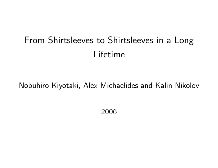
From Shirtsleeves to Shirtsleeves in a Long Lifetime Nobuhiro Kiyotaki, Alex Michaelides and Kalin Nikolov 2006

1 Question To what extent are ‡uctuations of housing prices and aggregate production consistent with fundamental conditions of technol- ogy and …nance? How does the life-cycle of consumption and home-ownership depend upon technology and limitation of contract enforce- ment?

We develop an overlapping generations model of a production economy in which land and capital are combined into residential and commercial structures. Each household chooses consump- tion and home-ownership under collateral constraints Idea: Household enjoys an owned house more than a rented house ! Hence wants to buy a house But, the household faces a collateral constraint and therefore needs to save for a downpayment ! Young and poor rent, rich and old own ! First order welfare e¤ects

Implications: Life-cycle of home-ownership depends upon � Technology: importance of land for production of structures growth rate of population and labor productivity � Financial system � Pension system

Change in growth rate of population and labor productivity a¤ect both level and growth rate of housing price and aggregate quantities Change in the level of labor productivity and required rate of return for foreigners a¤ects level of housing price and aggregate quantities Change in the downpayment requirement of housing has a lim- ited e¤ect on housing prices and aggregate output, even though it has a signi…cant e¤ect on the home-ownership rate

2 Model Output is produced from labor and productive structures Y t = F ( A t N t ; Z Y t ) = ( A t N t ) 1 � � Z � (1) Y t Capital and land form structures Z t = K � t L 1 � � (2) Capital accumulation through investment K t = �K t � 1 + I t (3)

Continuum of workers with population size of N t : High productivity workers " � m & 1 � ! 1 � � Medium productivity workers ! Retirees � ! Dead " � l G N � ! % � ! Low Productivity workers

Preferences hP 1 i t =0 � t u ( c t ; (1 � I ( rent )) h t ) E 0 (4) where 2 1 � � 3 1 � � 0 1 � 0 1 @ c h 6 7 u ( c; h ) = = (1 � � ) A @ A 4 5 1 � � �

Limited commitment Tenant cannot precommit to take proper care of rented house ! landlords limit the freedom of the tenants ! utility discount for tenants Potential hold-up between the owners of land and building ! must own capital and land together ! only asset traded is share of structures Borrowers may default ! only home-owner can borrow (issue outside equity) up to collateral fraction: s t � �h t : for a home-owner (5) s t � 0 : for a tenant

Flow-of-funds constraint For a worker c t + r t h t + q t s t = (1 � � ) w t " t + r t s t + d t s t � 1 (6) For a retiree c t + r t h t + q t s t = b t + r t s t + ( d t =� ) s t � 1 For the representative foreigner C � t + q t S � t = r t S � t + d t S � t � 1 The asset demand of the foreigner t = S � + � ( R t � R � S � t ) ; where d t +1 R t = (7) q t � r t

Representative …rm chooses the production plan ( Y t ; N t ; Z Y t ; Z t ; K t ; I t ) to maxi- mize the value of the …rm: V t = Y t � w t N t � r t Z Y t + r t Z t � I t + 1 E t V t +1 R t subject to the constraint of technology (1 ; 2 ; 3) : d t is gross dividend to the shareholder of structure from date t-1: d t Z t � 1 = V t

Market clearing Labor Z N t n t ( i ) di = " l N l t + " m N m t + " h N h t = N l t + N m t + N h N t = t 0 Goods Z N t c t ( i ) di + C � Y t = I t + t 0 Use of structures Z N t Z t = Z Y t + h t ( i ) di 0 Shares of structures Z N t Z t = S � t + s t ( i ) di 0

Behavior of representative …rm w t = (1 � � ) Y t =N t r t = �Y t =Z Y t 1 � � = �r t ( L=K t ) 1 � � R t V t = q t Z t � I t

Behavior of Households Indirect utility with net worth x and shareholding s : Tenant: s < �h 0 1 ( � � 1)(1 � � ) [ x � ( q � r ) s ] 1 � � r u T ( s; x ) = B C @ A 1 � 1 � � Constrained home-owner: s = �h 8 1 � � 9 2 3 � 2 3 1 � � > 4 x � ( q � r + r > > � ) s > 4 s=� < = u C ( s; x ) = 6 7 6 7 = (1 � � ) 5 5 > > > > � 1 � � : ; Unconstrained home-owner: s > �h u U ( s; x ) = r ( � � 1)(1 � � ) [ x � ( q � r ) s ] 1 � � 1 � �

Value function for the retiree V r ( x; A ) = Max f � � u T ( s; x ) + ��V r ( b 0 + ( d 0 =� ) s; A 0 ) max ; s � � u C ( s; x ) + ��V r ( b 0 + ( d 0 =� ) s; A 0 ) max ; s � � u U ( s; x ) + ��V r ( b 0 + ( d 0 =� ) s; A 0 ) max g s

Value function for worker with low productivity V l ( x; A ) = Max ( 8 9 u T ( s; x ) + � [( ! � � l ) V l ( � l w 0 + d 0 s; A 0 )+ > > > > < = max ; ; � l V m ( � m w m + d 0 s; A 0 ) + (1 � ! ) V r ( b 0 + d 0 s; A 0 ) > > s > > : 8 9 u C ( s; x ) + � [( ! � � l ) V l ( � l w 0 + d 0 s; A 0 )+ > > > > < = max ; � l V m ( � m w m + d 0 s; A 0 ) + (1 � ! ) V r ( b 0 + d 0 s; A 0 ) > > s > > : ; s 8 9 u U ( s; x ) + � [( ! � � l ) V l ( � l w 0 + d 0 s; A 0 )+ > > > > < = max ; ) � l V m ( � m w m + d 0 s; A 0 ) + (1 � ! ) V r ( b 0 + d 0 s; A 0 ) > > s > > : Value functions for medium productivity worker and high pro- ductivity worker are similarly de…ned

Steady state growth with productivity growth A t +1 = G A > A t 1 =G N Growth rate of aggregate output Y t +1 = C t +1 = I t +1 = K t +1 = G Y Y t C t I t K t Growth rate of aggregate structures Z t +1 = Z Y t +1 = G Z Z t Z Y t ! G Y = ( G A G N ) (1 � � ) = (1 � �� ) < G A G N if G A G N > 1 G Z = G � Y < G Y G r = r t +1 = q t +1 = G 1 � � > 1 Y r t q t

Table 1: Long run aggregate features of the U.S. economy 1900 1939 1958 Average Reproducible tangible assets/GDP 3.07 3.34 2.92 3.3 Land/GDP 1.61 0.96 0.66 - Net foreign assets/GDP -0.12 0.02 0.05 - Fraction of productive structures 0.47 0.43 0.42 0.53

Table 2: Home ownership rates in % 1970 1980 1990 2003 United States 64.2 65.6 64.0 68.3 Germany - 41.0 39.0 43.6 Italy - 59.0 68.0 80.0 United Kingdom 50.0 55.0 66.0 70.0 Japan - 60.0 61.0 62.0 Table 3: U.S. Home-Ownership Rates (in %) 1900 1920 1940 1960 1980 1990 whites 48.5 47.1 42.1 64.0 68.6 66.5 blacks 24.1 24.6 20.5 35.8 43.8 40.9

Baseline parameter values � = 0 : 26 : share of productive structures in output, � = 0 : 9 : share of capital in structures � = 0 : 75 : share of consumption of goods, = 0 : 09 : fraction of utility loss from renting a house, � = 0 : 3 : fraction of house that needs downpayment, � = 20 : sensitivity of foreign share demand " l = 0 : 33 ; " m = 0 : 663 ; " h = 2 : 65 : labor productivity, � l = 0 : 08 ; � m = 0 : 014 : probability of switching productivity, ! = 0 : 978 : probability of continuing working, � = 0 : 945 : probability of surviving, b=w = 0 : 2 : ratio of retirement bene…t to pretax average wage G A = 1 : 02 : labor productivity growth, G N = 1 : 01 : popula- tion growth rate

FIGURE 1A: Policy functions for a low productivity worker Home purchase 0.800 Housing 0.700 0.600 x1l x2l 0.500 Consumption 0.400 0.300 0.200 Unconstrained 0.100 0.000 0.000 0.500 1.000 1.500 2.000 2.500 3.000 3.500 FIGURE 1B: Evolution of savings for a low productivity household 0.500 Constrained home purchase 0.450 0.400 45deg line 0.350 0.300 0.250 s'=s(s,q,yl) 0.200 0.150 0.100 0.050 0.000 0.000 0.100 0.200 0.300 0.400 0.500

FIGURE 2A: Policy functions for a high productivity worker Home purchase 1.000 0.900 Housing 0.800 x2m x1m 0.700 0.600 0.500 Consumption 0.400 0.300 0.200 Unconstrained 0.100 0.000 0.000 0.500 1.000 1.500 2.000 2.500 3.000 3.500 FIGURE 2B: Evolution of savings for a high productivity household 2.500 Constrained home purchase 2.000 1.500 s'=s(s,q,ym) sm* 1.000 0.500 45deg line 0.000 0.000 0.500 1.000 1.500 2.000 2.500

FIGURE 3A: Policy functions for the Retiree 0.700 Home Purchase Housing 0.600 0.500 x1r x2r Consumption 0.400 0.300 0.200 Unconstrained 0.100 0.000 0.000 0.500 1.000 1.500 2.000 2.500 3.000 3.500 FIGURE 3B: Evolution of savings for the retiree 0.500 Constrained home purchase 0.450 0.400 45deg line 0.350 0.300 0.250 s'=s(s,q,b) sr* 0.200 0.150 0.100 0.050 0.000 0.000 0.100 0.200 0.300 0.400 0.500

FIGURE 4: An example life time Productivity increase, constrained house purchase 1.6 1.4 housing 1.2 1 0.8 shares 0.6 0.4 0.2 Unconstrained Retirement 0 1 5 9 13 17 21 25 29 33 37 41 45 49 53 57 61 65 69

Features of the steady state of baseline economy (detailed re- sults in table 5) ! Tenants - 25% of population Constrained - 8.3% of population ! Average house size relative to unconstrained Tenants - 34% Constrained - 22% ! Average shareholding relative to unconstrained Tenants - 0.08%

Constrained - 0.33% ! Price-rental ratio of housing - 8.65 years ! Real rate of returns on share in terms of output - 6.62%